Statistical concepts and market returns

1. Statistical concepts and market returns

2. Populations and samples The subset of data used in statistical inference is known as a sample and the larger body of data is known as the population. The population is defined as all members of the group in which we are interested. Sample Population

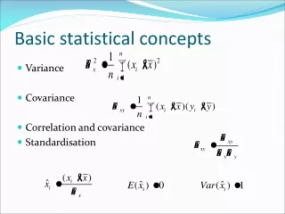
3. Parameters and Sample Statistics A population has parameters, and a sample has statistics. Descriptive statistics that characterize population values are called parameters. Examples: mean, median, mode, variance, skewness, kurtosis Descriptive statistics that characterize samples are known as sample statistics. Examples: sample mean, sample median, sample variance By convention, we often omit the term “sample” in front of sample statistics, a practice that can lead to confusion when discussing both the sample and the population.

4. Measurement Scales Statistical inference is affected by the type of data we are trying to analyze. Nominal scales categorize data but do not rank them. Examples: fund style, country of origin, manager gender Ordinal scales sort data into categories that are ordered with respect to the characteristic along which the scale is measured. Examples: “star” rankings, class rank, credit rating Interval scales provide both the relative position (rank) and assurance that the differences between scale values are equal. Example: temperature Ratio scales have all the characteristics of interval scales and a zero point at the origin. Examples: rates of return, corporate profits, bond maturity Weak Scales Strong Scales

5. Holding period returns Holding period returns are a fundamental building block of the statistical analysis of investments. Holding period returns (HPR) are calculated as the price at the end of the period plus any cash distribution during the period minus the beginning of period price, all divided by the beginning period price. For this stock, which is nondividend paying, the HPRs are:

6. Frequency distributions A tabular display of data summarized into intervals is known as a frequency distribution. Constructing a frequency distribution: Sort the data in ascending order. Calculate the range of the data, defined as Range = Maximum value – Minimum value. Decide on the number of intervals in the frequency distribution, k. Determine interval width as Range/k. Determine the intervals by successively adding the interval width to the minimum value to determine the ending points of intervals, stopping after reaching an interval that includes the maximum value. Count the number of observations falling in each interval. Construct a table of the intervals listed from smallest to largest that shows the number of observations falling in each interval.

7. Frequency Distributions Focus on: Holding Period Returns Suppose we have 12 holding period return observations from a non-dividend-paying stock, sorted in ascending order: −4.57, −4.04, −1.64, 0.28, 1.34, 2.35, 2.38, 4.28, 4.42, 4.68, 7.16, and 11.43. Using k = 4, we have intervals with width of 4. The resulting frequency distribution is

8. Relative and cumulative frequency Focus on: Holding Period Returns Relative frequency is the absolute frequency divided by the total number of observations. Cumulative (relative) frequency is the relative frequency of all observations occurring before a given interval. ÷ 12 + =

9. Histograms Focus on: Holding Period Returns Histograms are the graphical representation of a frequency distribution.

10. Frequency Polygon Focus on: Holding Period Returns Frequency polygons are often used to provide higher visual continuity than histograms.

11. Measures of central tendency These measures describe where the data are centered. Arithmetic Mean The arithmetic mean is the sum of the observations divided by the number of observations. Population mean  Sample mean  The sample mean is often interpreted as the fulcrum, or center of gravity, for a given set of data. Cross-sectional data occur across different observation types at one point in time, and time-series data occur for the same unit of observation across time. s s m

12. Measures of central tendency Focus on: Cross-Sectional Sample Mean Return Source: www.msci.com.

13. Measures of central tendency Mean as a center of gravity for the data object –31.25% –2.97% –44.05%

14. Measures of central tendency These measures also describe where the data are centered. Weighted Mean  The sum of the observations times each observation’s weight (proportional representation in the sample), where the weight is chosen to meet a statistical or financial goal. Example: Portfolio return Geometric Mean  Represents the growth rate or compounded return on an investment when Xis 1 + R Harmonic Mean  A weighted mean in which each observation’s weight is inversely proportional to its magnitude. Example: Cost averaging

15. Measures of central tendency These measures also describe where the data are centered. The median is the middle observation by rank. When we have an odd number of observations, the median will be the closest to the middle. When we have an even number, the median will be the average of the two middle values. The mode is the most frequently occurring value in a distribution. Distributions are unimodal when there is a single most frequently occurring value and multimodal if there is more than one frequently occurring value. Examples: Bimodal and trimodal Unimodal Bimodal

16. Measures of central tendency Focus on: Calculating a Median or Mode

17. Interval location measures Quantiles are values that identify the location of data at or below which specified proportions lie. Quartiles, Quintiles, Deciles, and Percentiles Quarters, fifths, tenths, and hundredths Py = 0.25 or 0.20 or 0.10 or 0.01 Sometimes, we may be able to determine the exact location because the percentile cutoff corresponds to an exact location in our data. Example: The quartile (25th percentile) of 60 observations is the 15th observation as rank-ordered. Sometimes, the ordering doesn’t lead to exact integer divisibility. Then, the position of percentile, Py, denoted as Ly, is found by and the value of Pyis found by linear interpolation.

18. Interval Location measures Focus on: First Quintile 

19. Weighted average Also known as a weighted mean, the most common application of this measure in investments is the weighted mean return to a portfolio. Consider again the country-level data. You have constructed a portfolio that has 50% of its weight in Portugal, Ireland, Greece, and Spain and 50% of its weight in Germany and the UK. Each of the first four countries is equally weighted within the 50%, as are Germany and the UK within their 50%. What is the weighted average return to the portfolio?

20. Measures of dispersion Dispersion measures variability around a measure of central tendency. If mean return represents reward, then dispersion represents risk. Range  Range = Maximum value – Minimum value The distance between the maximum value in the data and the minimum value in the data. For the country return data, the range is [–2.97% – (–44.05%)] = 41.08% Mean Absolute Deviation (MAD)  The arithmetic average of the absolute value of deviations from the mean. For the country return data, the MAD is 7.04%.

21. Measures of dispersion Dispersion measures variability around a measure of central tendency. If mean return represents reward, then dispersion represents risk. Variance is the average squared deviation from the mean. Population variance  Sample variance  Sample variance is “penalized” by dividing by n – 1 instead of n to account for the fact that the measure of central tendency used, , is an estimate of the true population parameter, m, and so has some uncertainty associated with it. Standard deviation is the square root of variance.

22. Measures of dispersion Focus on: Sample Standard Deviation

23. semivariance We are often concerned with measures of risk that focus on the “downside” of the possible outcomes—in other words, the losses. Semivariance is the average squared deviation below the mean. Semideviation is the square root of semivariance. Both are a measure of dispersion focusing only on those observations below the mean. Target semivariance, by analogy, is the average squared deviation below some specified target rate, B, and represents the “downside” risk of being below the target, B.

24. Chebyshev’s inequality This expression gives the minimum proportion of values, p, within k standard deviations of the mean for any distribution whenever k > 1.

25. Chebyshev’s inequality Focus on: Calculating Proportions Using Chebyshev’s Inequality For our country data, the mean is –31.25% and the sample standard deviation is 9.95%. Lower cutoff at 1.25 standard deviations: –31.25% – 1.25 (9.95%) = – 43.6875% Upper cutoff at 1.25 standard deviations: –31.25% + 1.25 (9.95%) = – 18.8125%

26. Combining risk and return Measures of relative dispersion are used to compare risk and return across differing sets of observations. The coefficient of variation is the ratio of the standard deviation of a set of observations to their mean value. This ratio can be thought of as the units of risk per unit of mean return. The Sharpe Ratio is the ratio of the mean excess return (mean return minus the mean risk-free rate) per unit of standard deviation. This ratio can be thought of as units of risky return (excess return) per unit of risk. This will also be the slope of a line in expected return/standard deviation space. E(r) Sp rf s

27. Combining risk and return Focus on: Coefficient of Variation and the Sharpe Ratio Consider a portfolio with a mean return of 25.26% and a standard deviation of returns of 9.95%. The coefficient of variation is If the risk-free rate is 3%, then the Sharpe Ratio is

28. Combining centrality, dispersion, and symmetry For a symmetrical distribution, the mean, median, and mode (if it exists) will all be at the same location. If the distribution is positively skewed, then the mean will be greater than the median, which will be greater than the mode (if it exists). If the distribution is negatively skewed, then the mean will be less than the median, which will be less than the mode (if it exists). mode < median < mean Example: Positive skew

29. Skewness The degree of symmetry in the dispersion of values around the mean is known as skewness. If observations are equally dispersed around the mean, the distribution is said to be symmetrical. If the distribution has a long tail on one side and a “fatter” distribution on the other side, it is said to be skewed in the direction of the long tail. Skew Right No Skew Skew Left

30. kurtosis Kurtosis measures the relative amount of “peakedness” as compared with the normal distribution, which has a kurtosis of 3. We typically express this measure in terms of excess kurtosis being the observed kurtosis minus 3. Distributions are referred to as being Leptokurtic (more peaked than the normal; fatter tails) Platykurtic (less peaked than the normal; thinner tails) or Mesokurtic (equivalent to the normal).

31. skewness and kurtosis Focus on: Sample Skewness Recall that a distribution with perfect symmetry has skewness of zero. Because cubing preserves the sign of the original difference between Xi and its mean, if deviations from the mean are equally distributed on each side of the mean, they will cancel each other out, leading to skewness of zero. If there are some very large values, they become even larger when cubed, and the skewness measure will then reflect this. Large negative values  Negative sample skewness Large positive value  Positive sample skewness

32. skewness and kurtosis Focus on: Sample Kurtosis Kurtosis measures the relative “peakedness” of the distribution. A leptokurtic distribution is more peaked than the normal distribution. More observations closer to the mean and out in the tails. Often known as having “fat tails.” A mesokurtic distribution has peakedness equal to the normal distribution. A platykurtic distribution is less peaked than the normal distribution. It is more evenly distributed across the range of possible values. The kurtosis of the normal distribution is 3; hence, excess kurtosis is sample kurtosis minus 3.

33. Summary The underlying foundation of statistically based quantitative analysis lies with the concepts of a sample versus a population. We use sample statistics to describe the sample and to infer information about its associated population. Descriptive statistics for samples and populations include measures of centrality, location, and dispersion, such as mean, range, and variance, respectively. We can combine traditional measures of return (such as mean) and risk (such as standard deviation) to measure the combined effects of risk and return using the coefficient of variation and the Sharpe Ratio. The normal distribution is of central importance in investments, and as a result, we often compare statistical properties, such as skewness and kurtosis, with those of the normal distribution.