Understanding Complexity in Climate Science

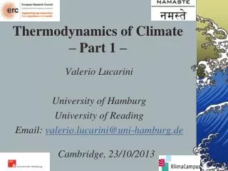
1. Thermodynamics of Climate – Part 1 – Valerio Lucarini Universityof Hamburg University of Reading Email: valerio.lucarini@uni-hamburg.de Cambridge, 23/10/2013

2. Climate and Physics • “A solved problem, just some well-known equations and a lot of integrations” • “who cares about the mathematical/physical consistency of models: better computers, better simulations, that’s it! • … where is the science? • “I regret to inform the author that geophysical problems related to climate are of little interest for the physical community…” • “Who cares of energy and entropy? We are interested in T, P, precipitation”

3. What’s a Complex system? • A complex system is a system composed of interconnected parts that, as a whole, exhibit one or more properties not obvious from the properties of the individual parts • Reductionism, whichhasplayed a fundamentalrole in develpoingscientificknowledge, isnotapplicable. • The Galileanscientificframeworkgiven by recurrentinterplay of experimentalresults (performed in a cenceptual/reallaboratoryprovided with a clock, a measuring and a recordingdevice), and theoreticalpredictionsischallenged

4. Some Properties of Complex Systems • Spontaneous Pattern formation • Symmetry break and instabilities • Irreversibility • Entropy Production • Variability of manyspatial and temporalscales • Non-trivialnumericalmodels • Sensitive dependence on initialconditions • limitedpredictability time

5. Complicated vs Complex • Not Complicated and Not Complex • Harmonic oscillator in 1D • Complicated and Not Complex • Gas of non-interacting oscillators (phonons) • Integrable systems are always not complex • Not Complicated and Complex • Lorenz 63 model has only 3 degrees of freedom • Complicated and Complex • Turbulent fluid, Society • ‘Complex’ comes from the past participle of the Latin verb complector, -ari(to entwine). • ‘Complicated’ comes from the past participle of the Latin verb complico, -are (to put together).

6. Map of Complexity • Climate Science is mysteriously missing!

7. Map of Complexity • Climate Science isperceivedasbeingtootechnical, political Climate Science

8. Some definitions • The climate system (CS) is constituted by four interconnected sub-systems:atmosphere, hydrosphere, cryosphere, and biosphere, • The sub-systems evolve under the action of macroscopic driving and modulating agents, such as solar heating, Earth’s rotation and gravitation. • The CS features many degrees of freedom • This makes it complicated • The CS features variability on many time-space scales and sensitive dependence on IC • This makes it complex. • The climate is defined as the set of the statistical properties of the CS.

9. Three major theoreticalchallenges in analysing the CS • Mathematics: In dynamicalsystems, the stabilityproperties of the time mean state saynothingabout the properties of the full nonlinearsystem • impossibility of defining a theory of the time-meanpropertiesrelyingonly on the time-meanfields. • Physics: Itisimpossible to apply the fluctuation-dissipationtheorem for a chaotic dissipative systemsuchas the climatesystem • non-equivalencebetween the external and internalfluctuationsClimateChangeis hard to parameterise • Numerics: Climateis a stiffproblem (verydifferent time scales) “optimal” resolution? • brute force approachisnotnecessarily the solution.

10. Three major experimental challenges in analysing the CS • Synchronic coherence of data • Data feature hugely varying degree of precision • Diachronic coherence of data • Technology and prescriptions for data collection have changed with time • Space-time coverage • Data density change with location (Antarctica vs Germany) • We have “direct” data only since Galileo time • Before, we have to rely on indirect (proxy) data • Unusual with respect to “typical” science

11. Scales of Motions(Stommel/Smagorinsky)

12. Atmospheric Motions • Three contrasting approaches: • Those who like maps, look for features/particles • Those who like regularity, look for waves • Those who like irreversibility, look for turbulence • Let’s see schematically these 3 visions of the world

13. Features/Particles • Focus is on specific (self)organised structures • Hurricane physics/track

14. Atmospheric (macro) turbulence • Energy, enstrophy cascades, 2D vs 3D Note: NOTHING is really 2D in the atmosphere

15. Waves in the atmosphere • Large and small scale patterns

16. “Waves” in the atmosphere? • Hayashi-Fraedrich decomposition

17. “Waves” in GCMs • GCMs differ in representation of large scale atmospheric processes • Just Kinematics? • What we see are only unstable waves and their effects

18. Evolution of Climate Models • With improvement of CPU and of scientificknowledge, CMshavegained new componentsdefinition of “climate” hasalsochanged

19. Full-blownClimate Model Since the ‘40s, some of largestcomputersare devoted to climate modelling

20. G O A L S O F M O D E L L I N G Local evolution in the phase space NWPvs.Statistical properties on the attractor Climate Modeling

21. Climate Models uncertainties • Uncertainties of the 1st kind • Are ourinitialconditionscorrect? Not so relevant for CM, crucial for NWP • Uncertainties of the 2nd kind • Are werepresentingall the mostrelevantprocesses for the scales of ourinterest? Are werepresentingthemwell? (structuraluncertainty) • Are ourheuristicparameters appropriate? (parametricuncertainty) • Uncertainty on the metrics: • Are wecomparingpropertly and in a meaningful way ouroutputs with the observational data?

22. Plurality of Models • In Climate Science, notonly full-blownmodels (most accurate representation of the largestnumber of processes) are used • Simplermodels are used to try to capture the structuralproperties of the CS • Lessexpensive, more flexible– parametricexploration • CMsuncertainties are addressed by comparing • CMs of similarcomplexity (horizontal) • CMsalong a hierarchicalladder (vertical) • The mostpowerfultoolisnot the most appropriate for allproblems, addressing the big picturerequires a variety of instruments • Allmodels are “wrong”! (butwe are notblind!)

24. Multimodel ensemble • Outputs of different models should not be merged: not different realisations of the same process in the world of metamodels (“large numbers law”) • Each model has a different attractor with different properties, they are different objects! • There is no good reason to assume that the model average is the best approximation of reality • Intensityof the hydrologicalcycle over the Danubebasin for IPCC4AR models for 1961-2000 (L. et al. 2008) • Purpleis EM: whatdoesittellus?

25. Probability • The epistemologypertaining to climate science impliesthatitsanswers must be plural and stated in probabilisticterms. • Here, parametricuncertainty for a given model isexplored • This PDF contains a hugeamount of info! • We can assessrisks, thisis an instrument of decision-making Webster et al. 2001

26. E N E R G Y TRANS P O R T

27. Energy & GW – Perfect GCM Forcing • NESS→Transient → NESS • Applies to the wholeclimate and to to allclimaticsubdomains • for atmosphereτis small, always quasi-equilibrated τ L. and Ragone, 2011 Total warming

28. Energy and GW –ActualGCMs L. and Ragone, 2011 • Not only bias: bias control ≠ bias final state • Bias depends on climate state!  Dissipation Forcing τ

29. Comments • “Well, we care about T and P, not Energy” • Troublesome, practically and conceptually • A steady state with an energy bias? • How relevant are projections related to forcings of the same order of magnitude of the bias? • In most physical sciences, one would dismiss entirely a model like this, instead of using it for O(1000) publications • Should we do the same? • Food for thought

30. PCMDI/CMIP3 GCMs - IPCC4AR • Pre-Industrial control runs (100 years) • SRESA1B 720 ppm CO2 stabilization (100 years, as far as possible from 2100)

31. PI – TOA Energy Balance IPCC4AR Models Control Run • Is the viscous loss of kinetic energy re-injected in the system? (Becker 03, L & Fraedrich 2009) L. and Ragone, 2011

32. PI – Atmosphere Energy Balance

33. PI – Ocean Energy Balance • PI – Ocean Energy Balance • Most models bias (typ. >0) is < 1 Wm-2 • Larger interannual variability than atmosphere • PI – Land Energy Balance • Thin (à la Saltzman) climate subsystem • Most models bias (typ. >0) is < 2 Wm-2 • Model 5 bias is 2 Wm-2; 10 Wm-2 excess for Model 19

34. ΔTOA Energy Balance • In 2200-2300 systemis out of equilibrium by additional O(1 Wm-2) • Mostexcessheatgoesinto the ocean (atmosphere, landunchanged) • Need for longerintegrations(τ >300y)

35. Estimated B(P-E) vs Total Runoff – (Annual)Results- XX Century Climate – (1961-2000)

36. Energy Imbalance

37. From Energy Balance to Transports • From energy conservation: • If we integrate vertically, zonally Transports Long term averages • If fluxes integrate globally to 0 – as they should – the T functions are zero at BOTH poles • Otherwise (relatively small!) biases • We compute annual meridional transports starting from annual TOA and surface zonally averaged fluxes • Can be done for TOA with satellites!

38. PI -Transports T A O Stone ‘78 constraint well obeyed

39. Max Transport - TOA 6 ° (2,3 gridpoints) 1.2 PW 20%

40. Max Transport - Atmosphere 0.8 PW 15% 4 °

41. Max Transport - Ocean 0.8 PW 50% 5 °

42. SRESA1B -Transports T A O

43. ΔAtm Transport • Increase of Atm Transport: LH effect

44. Δ peak NH Atm Transport • Poleward shift of Storm track: SH& NH

45. NH - Correlation btw A & O Transports • A negative correlation exists between the yearly maxima of atmospheric and oceanic transport • Compensating mechanism tends to become stronger with GW • About the same in the SH • Bjerknes compensation mechanism

46. Disequilibrium in the Earth system climate Multiscale (Kleidon, 2011)

47. Looking for the big picture • Global structural properties (Saltzman 2002). • Deterministic & stochastic dynamical systems • Example: stability of the thermohaline circulation • Stochastic forcing: ad hoc “closure theory” for noise • Stat Mech & Thermodynamic perspective • Planets are non-equilibrium thermodynamical systems • Thermodynamics: large scale properties of the climate system; definition of robust metrics for GCMs, data • Stat Mech for Climate response to perturbations EQ NON EQ 47

48. Thermodynamics of the CS • The CS generates entropy (irreversibility), produces kinetic energy with efficiency η(engine), and keeps a steady state by balancing fluxes with surroundings (Ozawa et al., 2003) • Fluid motions result from mechanical work, and re-equilibrate the energy balance. • Wehave a unifyingpictureconnecting the Energy cycle to the MEPP (L. 2009); • Thisapproachhelps for understandingmanyprocesses (L et al., 2010; Boschi et al. 2012): • Understandingmechanisms for climatetransitions; • Defininggeneralisedsensitivities • Proposingparameterisations

49. Concluding… • The CS seems to cover manyaspects of the science of complexsystems • Weknow a lotmore, a lotlessthanusuallyperceived • Surely, in order to perform a leap in understanding, weneed to acknowledge the differentepisthemologyrelevant for the CS and developsmart science tacklingfundamentalissues • “Shock and Awe” numericalsimulationsmayprovideonlyincrementalimprovements: heavysimulations are needed, butclimate science is NOT just a technologicalchallenge, weneed new ideas • I believethat non-equilibriumthermodynamics & statisticalmechanicsmay help devising new efficientstrategies to address the problems • Next time! Entropy, Efficiency, TippingPoints

50. Bibliography • Held, I.M., Bull. Amer. Meteor. Soc., 86, 1609–1614 (2005) • Hasson S.,, V. Lucarini, and S. Pascale, Earth Syst. Dynam. Discuss., 4, 109–177, 2013 • Lucarini, V., R. Danihlik, I. Kriegerova and A. Speranza. J. Geophys. Res., 113, D09107 (2008) • Peixoto J. and A. Oort, Physics of Climate (AIP, 1992) • Saltzman B., Dynamic Paleoclimatology (Academic Press, 2002) • Lucarini V., Validation of Climate Models, in Encyclopaedia of Global Warming and Climate Change, Ed. G. Philander, 1053-1057(2008) • V. Lucarini, F. Ragone, Rev. Geophys. 49, RG1001 (2011) • B. Liepert and M. Previdi, Inter-model variability and biases of the global water cycle in CMIP3 coupled climate models, ERL 7 014006 (2012)