Chapter 7 - Modeling Issues
Chapter 7 explores critical modeling issues in regression analysis, focusing on heterogeneity and the comparison between fixed and random effects estimators. It discusses the implications of omitted variables, attrition, selectivity bias, and non-ignorable missing data. The chapter emphasizes the importance of understanding jointly dependent variables and covariance structures while examining practical and theoretical identification challenges. Techniques for handling different types of data, including clustered observations, are also presented, along with a comparison of regression coefficients and estimators to improve model reliability and accuracy.

Chapter 7 - Modeling Issues
E N D
Presentation Transcript
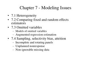
Chapter 7 - Modeling Issues • 7.1 Heterogeneity • 7.2 Comparing fixed and random effects estimators • 7.3 Omitted variables • Models of omitted variables • Augmented regression estimation • 7.4 Sampling, selectivity bias, attrition • Incomplete and rotating panels • Unplanned nonresponse • Non-ignorable missing data
7.1 Heterogeneity • Also think of clustering • different observations from the same subject (observational unit) tend to be related to one another. • Methods for handling this • variables in common • jointly dependent distribution functions
Variables in Common • These are latent (unobserved) variables • May be fixed (mean structure) or random (covariance structure) • May be organized by the cross-section or by time • If by cross-section, may be subject oriented (by i) or spatial • May be nested
Jointly Dependent Distribution Functions • For the covariance structures, this is a more general way to think about random variables that are common to subjects. • Also includes additional structures not suggested by the common variable approach • Example: For the error components model, we have Corr (yi1, yi2)= where >0. However, we need not require positive correlations for a general uniform correlation model.
Practical Identification with Heterogeneity may be difficult – Jones (1993) Example
Theoretical Identification with Heterogeneity may be Impossible– Neyman Scott (1948) Example • Example - Identification of variance components • Consider the fixed effects panel data model yit = i + it , i=1, …, n, t=1,2, • where Var it = 2 and Cov (i1, i2) = 2. • The ordinary least squares estimator of iis = (yi1+ yi2)/2. • Thus, the residuals are = (yi1- yi2)/2 and = (yi2- yi1)/2= - ei1 . • Thus, cannot be estimated, despite having 2n - n = n degrees of freedom available for estimating the variance components.
Estimation of regression coefficients without complete identification is possible • If our main goal is to estimate or test hypotheses about the regression coefficients, then we do not require knowledge of all aspects of the model. • For example, consider the one-way fixed effects model yi = i1i + Xiβ + i . • Apply the common transformation matrix Q = I – T -1J to each equation to get yi* = Q yi = QXi β + Qi = Xi*β + i*, • because Q 1 = 0. • Use ols on the transformed data. For T = 2, • Note that can estimate the quantity s 2 (1-r) yet cannot separate the terms s 2 and r.
7.2 Comparing fixed and random effects estimators • Sometimes, the context of the problem does not make clear the choice of fixed or random effects estimators. • It is of interest to compare the fixed effects to the random effects estimators using the data. • In random effects models, we assume that { ai } are independent of {eit} . • Think instead of drawing {xit } at random and performing inference conditional on {xit }. • Interpret {ai} to be the unobserved (time-invariant) characteristics of a subject. • This assumes that individual effects { ai} are independent of other individual characteristics {xit}, our strict conditional exogeneity assumption SEC6.
A special case • Consider the error components model with K = 2 so that yit = i + 0+ 1xit,1 + it , • We can express (Fuller-Battese) the gls estimator as • where • As20, we have that xit* xit,,yit* yit and b1,ECb1,OLS • As2 , we have that b1,ECb1,FE
A special case • Define the so-called “between groups” estimator, • This estimator can be motivated by averaging all observations from a subject and then computing an ordinary least squares estimator using the data . • The following decomposition due to Maddala (1971), b1,EC = (1- ) b1,FE + b1,B • where • measures the relative precision of the two estimators of .
A special case • To express the relationship between iand xi, we consider E [i| xi ]. • Specifically, we assume that i= i + , where {i} is i.i.d. • Thus, the model of correlated effects is yit = i + 0+ 1xit,1 + + it . • Surprisingly, one can show that the generalized least squares estimator of 1 is b1,FE. • Intuitively, by considering deviations from the time series means, , the fixed effects estimator “sweeps out” all time-constant omitted variables. • In this sense, the fixed effects estimator is robust to this type of model aberration. • Under the correlated effects model, • the estimator b1,FE is unbiased, consistent and asymptotically normal. • the estimators b1,HOM, b1,B and b1,EC are biased and inconsistent.
A special case • To test whether or not to use the random or fixed estimator, we need only examine the null hypothesis H0: = 0. • This is customarily done using the Hausman (1978) test statistic • This test statistic has an asymptotic (as n) chi-square distribution with 1 degree of freedom. • Test statistic is large, go with the fixed effects estimator • Test statistic is small, go with the random effects estimator
General Case • Assume that E αi = α and re-write the model as yi = Ziα + Xiβ + i* , • where i* = i + Zi (αi - α) and • Var i* = ZiD Zi + Ri = Vi. • This re-writing is necessary to make the beta’s under fixed and random effects formulations comparable. • With the appropriate definitions, the extension of Maddala’s (1971) result is • where • The extension of the Hausman test statistic is
Case study: Income tax payments • Consider the model with Variable Intercepts but no Variable Slopes (Error Components) • The test statistic is = 6.021 • With K = 8 degrees of freedom, the p-value associated with this test statistic is . • For the model with Variable Intercepts and two Variable Slopes • The test statistic is = 13.628. • With K = 8 degrees of freedom, the p-value associated with this test statistic is Prob( >13.628)=0.0341. .
7.3 Omitted Variables • I call these models of “correlated effects.” • Section 7.2 described the Hausman/Mundlak model of time-constant omitted variables. • Chamberlain (1982) – an alternative hypothesis • Omitted variables need not be time-constant • Hausman and Taylor (1981) – another alternative hypothesis • Some of the explanatory variables are not correlated with ai . • To estimate these models, Arellano (1993) used an “augmented” regression model. We will also use this approach. • For a different approach, Stata has programmed an instrumental variable approach introduce by Hausman and Taylor as well as Amemiya and Mac Curdy.
Unobserved Variables Models • Introduced by Palta and Yao (1991) and co-workers. • Let oi =(zi´, xi´)´ be observed variables and ui be “unobserved” variables. • Assuming multivariate normality, we can express:
Unobserved Variables Models • The unobserved variables enter the likelihood through: • linear conditional expectations (g) • correlation between observed and unobserved variables (Suo) • The fixed effects estimator may be biased, unlike the correlated effects model case. • By examining certain special cases, we again arrive at the Mundlak, Chamberlain and Hausman/Taylor alternative hypotheses. • Other alternatives are also of interest. Specifically, an “extended” Mundlak alternative is:
Examples of Correlated Effects Models • Assuming q = 1 and zit =1, this is Chamberlain’s alternative. • Chamberlain used the hypothesis: • Thus, • Assume an error components design for the x’s. That is, • Assuming q = 1 and zit =1, this is Mundlak’s alternative. That is • Further assume that the first K-rx-variables are uncorrelated with ai . This is the Hausman/Taylor alternative.
Augmented Regression Estimation and Testing • I advocate the “augmented” regression approach that uses the model: E [yi | hioi] = Zi hi + Xib + Gig. • Random slopes hithat do not affect the conditional regression function. • Thus, so that E [yi | oi] = Xib + Gig. • Choose Gi = G(Xi, Zi) to be a known function of the observed effects. • Choice of G depends on the alternative model you consider. • The test for omitted variables is thus H0: g = 0. • Define bAR and gAR to be the corresponding weighted least squares estimators.
Some Results • The estimator bAR is unbiased (even in the presence of omitted variables). • The weights corresponding to gls (Wi = Vi) and • yields bAR = bFE. • This is an extension of Mundlak’s alternative. • The chi-square test for H0: g = 0 is:
Determinants of Tax Liability • I examine a 4 % sample (258) of taxpayers from the University of Michigan/Ernst & Young Tax Data Base • The panel consists of tax years 1982-84, 86, 87 • Tax Liability data, we use • xit’b = linear function of demographic and earning characteristics of a taxpayer • zit’ai= a1i + a2i LNTPIit + a3i MRit • yit = logarithmic tax liability for the ith taxpayer in the tth year
Empirical Fits • I present fits of four different models • Random effects • includes variable intercept plus two variable slopes • +omitted variable corrections • Random coefficients • With AR1 parameter • effects +omitted variable corrections (“Extended Mundlak alternative”)
Results • Section 7.2 indicated, with only variable intercepts, that the fixed effects estimator is preferable to the random effects estimator. • For random effects, • two additional variable slope terms were useful • the random coefficients model did not yield a positive definite estimate of Var a, I used a third order factor analytic model • New tests indicate that both the fixed effects model with 3 variable components and the extended Mundlak model are preferable to the random effects model with 3 variable components • Comparing fixed effects model with 3 variable components and the extended Mundlak model, the AIC favors the former yet I advocate the latter (parsimony and so on).
7.4 Sampling, selectivity bias and attrition • 7.4.1 Incomplete and rotating panels • Early longitudinal and panel data methods assumed balanced data, that is, Ti = T. • This suggests techniques from multivariate analysis. • Data may not be available due to: • Delayed entry • Early exit • Intermittent nonresponse • If planned, then there is generally no difficulty. • See the text for the algebraic transformation needed. • Planned incomplete data is the norm in panel surveys of people.
7.4.2 Unplanned nonresponse • Types of panel survey nonresponse (source Verbeek and Nijman, 1996) • Initial nonresponse. A subject contacted cannot, or will not, participate. Because of limited information, this potential problem is often ignored in the analysis. • Unit nonresponse. A subject contacted cannot, or will not, participate even after repeated attempts (in subsequent waves) to include the subject. • Wave nonresponse. A subject does not respond for one or more time periods but does respond in the preceding and subsequent times (for example, the subject may be on vacation). • Attrition. A subject leaves the panel after participating in at least one survey.
Missing data models • Let rij be an indicator variable for the ijth observation, with a one indicating that this response is observed and a zero indicating that the response is missing. • Let ri = (ri1, …, riT) and r = (r1, …, rn). • The interest is in whether or not the responses influence the missing data mechanism. • Use yi = (yi1, …, yiT) to be the vector of all potentially observed responses for the ith subject • Let Y = (y1, …, yn)to be the collection of all potentially observed responses.
Rubin’s (1976) Missing data models • Missing completely at random (MCAR). • The case where Y does not affect the distribution of r. • Specifically, the missing data are MCAR if f(r | Y) = f(r), where f(.) is a generic probability mass function. • Little (1995) - the adjective “covariate dependent” is added when • Y does not affect the distribution of r, conditional on the covariates. • If the covariates are summarized as {X, Z}, then the condition corresponds to the relation f(r | Y, X, Z) = f(r| X, Z). • Example: x=age, y=income. Missingness could vary by income but is really due to age (young people don’t respond)
General advice on missing at random • One option is to treat the available data as if nonresponses were planned and use unbalanced estimation techniques. • Another option is to utilize only subjects with a complete set of observations by discarding observations from subjects with missing responses. • A third option is to impute values for missing responses. • Little and Rubin note that each option is generally easy to carry out and may be satisfactory with small amounts of missing data. • However, the second and third options may not be efficient. • Further, each option implicitly relies heavily on the MCAR assumption.
Selection Model • Partition the Y vector into observed and missing components: Y = (Yobs, Ymiss). • Selection model is given by f(r | Y). • With parameters θ and ψ, assume that the log likelihood of the observed random variables is L(θ,ψ) = log f(r, Yobs,θ,ψ) = log f(Yobs,θ) + log f(r | Yobs,ψ). • MCAR case • f(r | Yobs,ψ) = f(r | ψ) does not depend on Yobs. • Data missing at random (MAR) • if selection mechanism model distribution does not depend on Ymiss but may depend on Yobs. • That is, f(r | Y) = f(r | Yobs). • For both MAR and MCAR, the likelihood may be maximized over the parameters separately in term. • For inference about θ, the selection model mechanism may be “ignored.” • MAR and MCAR are referred to as the ignorable case.
Example – Income tax payments • Let y = tax liability and x = income. • The taxpayer is not selected (missing) with probability . • The selection mechanism is MCAR. • The taxpayer is not selected if tax liability < $100. • The selection mechanism depends on the observed and missing response. The selection mechanism cannot be ignored. • The taxpayer is not selected if income < $20,000. • The selection mechanism is MCAR, covariate dependent. • Assuming that the purpose of the analysis is to understand tax liabilities conditional on knowledge of income, stratifying based on income does not serious bias the analysis. • The probability of a taxpayer being selected decreases with tax liability. For example, suppose the probability of being selected is logit (-yi). • In this case, the selection mechanism depends on the observed and missing response. The selection mechanism cannot be ignored. • The taxpayer is followed over T = 2 periods. In the second period, a taxpayer is not selected if the first period tax < $100. • The selection mechanism is MAR. That is, the selection mechanism is based on an observed response.
Example - correction for selection bias • Historical heights. y = the height of men recruited to serve in the military. • The sample is subject to censoring in that minimum height standards were imposed for admission to the military. • The selection mechanism is non-ignorable because it depends on the individual’s height. • The joint distribution for observables is • f(r, Yobs, , ) = f(Yobs, , ) f(r | Yobs ) • This is easy to maximize in and . • If one ignored the censoring mechanisms, then the “log likelihood” is • MLEs based on this are different, and biased.
Non-ignorable missing data • There are many models of missing data mechanisms - see Little and Rubin (1987). • Heckman two-stage procedure • Heckman (1976) developed for cross-sectional data but also applicable to fixed effects panel data models. • Thus, use yit = i + xit β + it . • Further, assume that the sampling response mechanism is governed by the latent (unobserved) variable rit* rit* = wit γ+ hit . • We observe
Assume {yit, rit} is multivariate normal to get E (yit | rit* 0) = i + xit β + (wit γ), • where = and . • Heckman’s two-step procedure • Use the data {( rit, wit)} and a probit regression model to estimate γ. Call this estimator gH. • Use the estimator gH to create a new explanatory variable, xit,K+1 = (wit gH). • Run a one-way fixed effects model using the K explanatory variables xit as well as the additional explanatory variable xit,K+1. • To test for selection bias, test H0: = 0 . • Estimates of give a “correction for the selection bias.”
Hausman and Wise procedure • Use an error components model, yit = ai + xit β + it. • The sampling response mechanism is governed by the latent variable error components model rit* = xi + wit γ + hit . • The variances are: • if sax = sh = 0, then the selection process is independent of the observation process.
Hausman and Wise procedure • Again, assume joint normality. With this assumption, one can check that: • where git = E (xi + hit | ri). • Calculating this quantity is computationally intensive, requiring numerical integration of multivariate normals. • if sax = sh = 0, then E (yit | ri) = xit β.

