From last lecture
250 likes | 274 Vues
Learn about constructing simple lattices like boolean logic and powerset, utilizing combinatorial techniques to create more complex structures. Understand the concepts of May vs. Must analysis and the direction of flow functions in backward problems. Explore the theory of backward analyses and the precision concerns in computations with examples. Delve into path-sensitivity issues and explore the concept of Meet Over All Paths (MOP) in dataflow analysis. Examine path pruning, branch correlations, and meet over all feasible paths for enhanced precision in dataflow algorithms.

From last lecture
E N D
Presentation Transcript
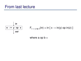
From last lecture in Fx := y op z(in) = in [ x ! in(y) op in(z) ] where a op b = x := y op z out
General approach to domain design • Simple lattices: • boolean logic lattice • powerset lattice • incomparable set: set of incomparable values, plus top and bottom (eg const prop lattice) • two point lattice: just top and bottom • Use combinators to create more complicated lattices • tuple lattice constructor • map lattice constructor
May vs Must • Has to do with definition of computed info • Set of x ! y must-point-to pairs • if we compute x ! y, then, then during program execution, x must point to y • Set of x! y may-point-to pairs • if during program execution, it is possible for x to point to y, then we must compute x ! y
Direction of analysis • Although constraints are not directional, flow functions are • All flow functions we have seen so far are in the forward direction • In some cases, the constraints are of the form in = F(out) • These are called backward problems. • Example: live variables • compute the of variables that may be live
Example: live variables • Set D = • Lattice: (D, v, ?, >, t, u) =
Example: live variables • Set D = 2 Vars • Lattice: (D, v, ?, >, t, u) = (2Vars, µ, ; ,Vars, [, Å) in Fx := y op z(out) = x := y op z out
Example: live variables • Set D = 2 Vars • Lattice: (D, v, ?, >, t, u) = (2Vars, µ, ; ,Vars, [, Å) in Fx := y op z(out) = out – { x } [ { y, z} x := y op z out
Example: live variables x := 5 y := x + 2 y := x + 10 x := x + 1 ... y ...
Example: live variables x := 5 y := x + 2 y := x + 10 x := x + 1 ... y ...
Revisiting assignment in Fx := y op z(out) = out – { x } [ { y, z} x := y op z out
Revisiting assignment in Fx := y op z(out) = out – { x } [ { y, z} x := y op z out
Theory of backward analyses • Can formalize backward analyses in two ways • Option 1: reverse flow graph, and then run forward problem • Option 2: re-develop the theory, but in the backward direction
Precision • Going back to constant prop, in what cases would we lose precision?
Precision • Going back to constant prop, in what cases would we lose precision? if (...) { x := -1; } else x := 1; } y := x * x; ... y ... if (p) { x := 5; } else x := 4; } ... if (p) { y := x + 1 } else { y := x + 2 } ... y ... x := 5 if (<expr>) { x := 6 } ... x ... where <expr> is equiv to false
Precision • The first problem: Unreachable code • solution: run unreachable code removal before • the unreachable code removal analysis will do its best, but may not remove all unreachable code • The other two problems are path-sensitivity issues • Branch correlations: some paths are infeasible • Path merging: can lead to loss of precision
MOP: meet over all paths • Information computed at a given point is the meet of the information computed by each path to the program point if (...) { x := -1; } else x := 1; } y := x * x; ... y ...
MOP • For a path p, which is a sequence of statements [s1, ..., sn] , define: Fp(in) = Fsn( ...Fs1(in) ... ) • In other words: Fp = • Given an edge e, let paths-to(e) be the (possibly infinite) set of paths that lead to e • Given an edge e, MOP(e) = • For us, should be called JOP...
MOP vs. dataflow • As we saw in our example, in general,MOP dataflow • In what cases is MOP the same as dataflow? Dataflow MOP x := -1; y := x * x; ... y ... x := 1; y := x * x; ... y ... x := -1; x := 1; Merge y := x * x; ... y ... Merge
MOP vs. dataflow • As we saw in our example, in general,MOP dataflow • In what cases is MOP the same as dataflow? • Distributive problems. A problem is distributive if: 8 a, b . F(a t b) = F(a) t F(b)
Summary of precision • Dataflow is the basic algorithm • To basic dataflow, we can add path-separation • Get MOP, which is same as dataflow for distributive problems • Variety of research efforts to get closer to MOP for non-distributive problems • To basic dataflow, we can add path-pruning • Get branch correlation • To basic dataflow, can add both: • meet over all feasible paths
Representing programs • Goals
Representing programs • Primary goals • analysis is easy and effective • just a few cases to handle • directly link related things • transformations are easy to perform • general, across input languages and target machines • Additional goals • compact in memory • easy to translate to and from • tracks info from source through to binary, for source-level debugging, profilling, typed binaries • extensible (new opts, targets, language features) • displayable