Introduction to Logistic Regression In Stata
581 likes | 1.11k Vues
Introduction to Logistic Regression In Stata. Maria T. Kaylen, Ph.D. Indiana Statistical Consulting Center WIM Spring 2014 April 11, 2014, 3:00-4:30pm. The Data/Research Question. Logistic regression is used when the dependent variable is binary. Typical coding:

Introduction to Logistic Regression In Stata
E N D
Presentation Transcript
Introduction to Logistic Regression In Stata Maria T. Kaylen, Ph.D. Indiana Statistical Consulting Center WIM Spring 2014 April 11, 2014, 3:00-4:30pm
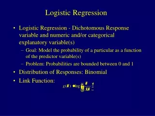
The Data/Research Question • Logistic regression is used when the dependent variable is binary. • Typical coding: 0 for negative outcome (event did not occur) 1 for positive outcome (event did occur) • Use this when you are interested in seeing how the independent variables affect the probability of the event occurring (or not occurring).
Examples • What demographic factors are related to whether or not someone votes in an election? • What circumstances affect the likelihood of someone being found guilty of a crime? • Do standardized test scores, high school grades, and social factors affect whether or not someone graduates from college?
Why Not Fit a Linear Model? • Example from UCLA’s Institute for Digital Research and Education website • Data: 1200 CA high schools, measuring achievement • DV: hiqual (high quality school or not, 0/1) • IV: avg_ed (average education of parents, 1-5) • Blue, “fitted values” are the predicted values from an OLS model • Red values are observed in the data • Problems: Negative values, values between 0 and 1
A Better Model • Blue line is the probability of hiqual=1 from the logistic regression model • Red values are observed in the data • Data fit is vastly improved • Predicted probabilities between 0 and 1 • Fits the observed data better
What is logistic regression? • Binary regression models typically take the form of probit or logit models. • The models are similar but the assumptions about the error distribution are different. • Probit: ε has mean=0 and variance=1 • Logit: ε has mean=0 and variance= • These assumptions about the error variance lead to the simple form of the probit and logit models.
Logistic Regression Model • This is a nonlinear model • A given change in x will often have less impact when Pr(y=1|x) is close to the extremes (0 or 1) compared to middle values. • Buying new or used car (from Agresti 2002) • Increasing family income by $50,000 would have less effect if x=$1,000,000 (for which Pr(y=1|x) is near 1) compared to x=$50,000
Interpreting Coefficients • A positive coefficient, , indicates that higher levels of x are associated with an increase in Pr(y=1|x). • A negative coefficient indicates that higher levels of x are associated with a decrease in Pr(y=1|x). • When =0, y and x are independent of one another.
Interpreting Coefficients • A one unit change in x is associated with the logit changing by , holding all other variables constant. • This isn’t very intuitive. • The odds of y=1 increase multiplicatively by for a one unit increase in x, holding all other variables constant. • is the odds ratio
Interpreting Coefficients • For positive , “the odds are times larger” or “the odds increase by a factor of ” • For negative , “the odds are times smaller” or “the odds decrease by a factor of ” • Values of close to 1 indicate a small change • Multiplying by 1.01 or 0.99 does not change the odds much!
Logit Command in Stata Logitdep_varind_vars Note 1: If you select a dependent variable that isn’t already coded as binary, Stata will define var=0 as 0 and all other values as 1. Note 2: Stata uses listwise deletion meaning that if a case has a missing value for any variable in the model, the case will be removed from the analysis.
Logit Output . logit ER stranger age i.income Iteration 0: log likelihood = -2227.7515 Iteration 1: log likelihood = -2192.8024 Iteration 2: log likelihood = -2192.1977 Iteration 3: log likelihood = -2192.1975 Logistic regression Number of obs = 5503 LR chi2(5) = 71.11 Prob > chi2 = 0.0000 Log likelihood = -2192.1975 Pseudo R2 = 0.0160 -------------------------------------------------------------------------------- ER | Coef. Std. Err. z P>|z| [95% Conf. Interval] ---------------+---------------------------------------------------------------- stranger | .3383692 .0833018 4.06 0.000 .1751007 .5016377 age | .0149814 .0026882 5.57 0.000 .0097127 .0202501 | income | Low Income | -.188747 .0916493 -2.06 0.039 -.3683764 -.0091176 Middle Income | -.4270387 .1274591 -3.35 0.001 -.6768539 -.1772235 High Income | -.5189086 .1362384 -3.81 0.000 -.7859309 -.2518862 | _cons | -2.20777 .1039755 -21.23 0.000 -2.411558 -2.003982 --------------------------------------------------------------------------------
SPost • J. Scott Long and Jeremy Freese wrote a program, SPost, that helps with interpreting results of categorical data analysis in Stata. • To install it, finditspostado
Logit Command Logitdep_varind_vars, or • The option, or, reports the odds ratios () for each independent variable. Standard errors and confidence intervals are also transformed. Logit dep_varind_vars, listcoef • The option, listcoef, reports additional variations of the coefficient (more on this later). Listcoef, reverse • This optioncalculates the inverse effects on the odds of the event in order to give you the odds of the event not occurring. Listcoef, percent • This option reports the percent change in the odds.
Logit, OR Output . xi: svy: logit ER stranger age i.income, or i.income _Iincome_1-4 (naturally coded; _Iincome_1 omitted) (running logit on estimation sample) Survey: Logistic regression Number of strata = 161 Number of obs = 5503 Number of PSUs = 314 Population size = 17385599 Design df = 153 F( 5, 149) = 12.00 Prob > F = 0.0000 ------------------------------------------------------------------------------ | Linearized ER | Odds Ratio Std. Err. t P>|t| [95% Conf. Interval] -------------+---------------------------------------------------------------- stranger | 1.343712 .1229243 3.23 0.002 1.121544 1.609889 age | 1.016358 .0026884 6.13 0.000 1.011061 1.021683 _Iincome_2 | .8592334 .0878709 -1.48 0.140 .7020493 1.05161 _Iincome_3 | .6947794 .1043255 -2.43 0.016 .5164337 .9347152 _Iincome_4 | .6243798 .0879345 -3.34 0.001 .4727311 .8246763 _cons | .1068197 .0112196 -21.29 0.000 .0868029 .1314525 ------------------------------------------------------------------------------ Note: strata with single sampling unit centered at overall mean.
Logit, OR Output ------------------------------------------------------------------------------ | Linearized ER | Odds Ratio Std. Err. t P>|t| [95% Conf. Interval] -------------+---------------------------------------------------------------- stranger | 1.343712 .1229243 3.23 0.002 1.121544 1.609889 age | 1.016358 .0026884 6.13 0.000 1.011061 1.021683 _Iincome_2 | .8592334 .0878709 -1.48 0.140 .7020493 1.05161 _Iincome_3 | .6947794 .1043255 -2.43 0.016 .5164337 .9347152 _Iincome_4 | .6243798 .0879345 -3.34 0.001 .4727311 .8246763 _cons | .1068197 .0112196 -21.29 0.000 .0868029 .1314525 ------------------------------------------------------------------------------ Note: strata with single sampling unit centered at overall mean. • The odds of victims going to the ER increase by a factor of 1.34when the offender is a stranger compared to a non-stranger, holding other variables constant (p<.01). • The odds of victims going to the ER increase by a factor of 1.02 for a one year increase in age, holding other variables constant (p<.01). • The odds of victims going to the ER decrease by a factor of0.69for middle income victims compared to lowest income victims, holding other variables constant (p<.05).
Listcoef • : factor change in the odds for a unit increase in x (odds ratio) • : factor change in the odds for a standard deviation increase in X • : standard deviation of X
Listcoef Output . listcoef, help logit (N=5503): Factor Change in Odds Odds of: ER vs No_ER ---------------------------------------------------------------------- ER | b z P>|z| e^be^bStdXSDofX -------------+-------------------------------------------------------- stranger | 0.29544 3.229 0.001 1.3437 1.1437 0.4544 age | 0.01623 6.134 0.000 1.0164 1.2408 13.2954 _Iincome_2 | -0.15171 -1.484 0.138 0.8592 0.9329 0.4580 _Iincome_3 | -0.36416 -2.425 0.015 0.6948 0.8812 0.3472 _Iincome_4 | -0.47100 -3.344 0.001 0.6244 0.8557 0.3308 ---------------------------------------------------------------------- b = raw coefficient z = z-score for test of b=0 P>|z| = p-value for z-test e^b = exp(b) = factor change in odds for unit increase in X e^bStdX = exp(b*SD of X) = change in odds for SD increase in X SDofX = standard deviation of X
Listcoef Output ---------------------------------------------------------------------- ER | b z P>|z| e^be^bStdXSDofX -------------+-------------------------------------------------------- stranger | 0.29544 3.229 0.001 1.3437 1.1437 0.4544 age | 0.01623 6.134 0.000 1.0164 1.240813.2954 _Iincome_2 | -0.15171 -1.484 0.138 0.8592 0.9329 0.4580 _Iincome_3 | -0.36416 -2.425 0.015 0.6948 0.8812 0.3472 _Iincome_4 | -0.47100 -3.344 0.001 0.6244 0.8557 0.3308 ---------------------------------------------------------------------- b = raw coefficient z = z-score for test of b=0 P>|z| = p-value for z-test e^b = exp(b) = factor change in odds for unit increase in X e^bStdX = exp(b*SD of X) = change in odds for SD increase in X SDofX = standard deviation of X • The odds of the victim going to the ER increase by a factor of 1.24 for a standard deviation increase in age (13.3 years), holding other variables constant (p<.01).
Listcoef, reverse Output . listcoef, help reverse logit (N=5503): Factor Change in Odds Odds of: No_ER vs ER ---------------------------------------------------------------------- ER | b z P>|z| e^be^bStdXSDofX -------------+-------------------------------------------------------- stranger | 0.29544 3.229 0.001 0.7442 0.8744 0.4544 age | 0.01623 6.134 0.000 0.9839 0.8060 13.2954 _Iincome_2 | -0.15171 -1.484 0.138 1.1638 1.0720 0.4580 _Iincome_3 | -0.36416 -2.425 0.015 1.4393 1.1348 0.3472 _Iincome_4 | -0.47100 -3.344 0.001 1.6016 1.1686 0.3308 ---------------------------------------------------------------------- b = raw coefficient z = z-score for test of b=0 P>|z| = p-value for z-test e^b = exp(b) = factor change in odds for unit increase in X e^bStdX = exp(b*SD of X) = change in odds for SD increase in X SDofX = standard deviation of X
Listcoef, reverse Output ---------------------------------------------------------------------- ER | b z P>|z| e^be^bStdXSDofX -------------+-------------------------------------------------------- stranger | 0.29544 3.229 0.001 0.7442 0.8744 0.4544 age | 0.01623 6.134 0.000 0.9839 0.8060 13.2954 _Iincome_2 | -0.15171 -1.484 0.138 1.1638 1.0720 0.4580 _Iincome_3 | -0.36416 -2.425 0.015 1.4393 1.1348 0.3472 _Iincome_4 | -0.47100 -3.344 0.001 1.6016 1.1686 0.3308 ---------------------------------------------------------------------- b = raw coefficient z = z-score for test of b=0 P>|z| = p-value for z-test e^b = exp(b) = factor change in odds for unit increase in X e^bStdX = exp(b*SD of X) = change in odds for SD increase in X SDofX = standard deviation of X • The odds of the victim not going to the ER increase by a factor of 1.60 for high income victims compared to lowest income victims, holding other variables constant (p<.01).
Listcoef, percent Output . listcoef, help percent logit (N=5503): Percentage Change in Odds Odds of: ER vs No_ER ---------------------------------------------------------------------- ER | b z P>|z| % %StdXSDofX -------------+-------------------------------------------------------- stranger | 0.29544 3.229 0.001 34.4 14.4 0.4544 age | 0.01623 6.134 0.000 1.6 24.1 13.2954 _Iincome_2 | -0.15171 -1.484 0.138 -14.1 -6.7 0.4580 _Iincome_3 | -0.36416 -2.425 0.015 -30.5 -11.9 0.3472 _Iincome_4 | -0.47100 -3.344 0.001 -37.6 -14.4 0.3308 ---------------------------------------------------------------------- b = raw coefficient z = z-score for test of b=0 P>|z| = p-value for z-test % = percent change in odds for unit increase in X %StdX = percent change in odds for SD increase in X SDofX = standard deviation of X
Listcoef, percent Output ---------------------------------------------------------------------- ER | b z P>|z| % %StdXSDofX -------------+-------------------------------------------------------- stranger | 0.29544 3.229 0.001 34.4 14.4 0.4544 age | 0.01623 6.134 0.000 1.6 24.1 13.2954 _Iincome_2 | -0.15171 -1.484 0.138 -14.1 -6.7 0.4580 _Iincome_3 | -0.36416 -2.425 0.015 -30.5 -11.9 0.3472 _Iincome_4 | -0.47100 -3.344 0.001 -37.6 -14.4 0.3308 ---------------------------------------------------------------------- b = raw coefficient z = z-score for test of b=0 P>|z| = p-value for z-test % = percent change in odds for unit increase in X %StdX = percent change in odds for SD increase in X SDofX = standard deviation of X • The odds of the victim going to the ER increase by 34.4% when the offender is a stranger compared to a non-stranger, holding other variables constant (p<.01).
Survey Weights • Survey data often come with survey weights that are needed to adjust the standard errors of the estimates. • You can use Stata’s survey commands with logit but not with all of the extra commands. SvysetPSU [weight] [,design options]
Predict *Note: Not allowed with svy Predict rstd, rs • After running the logit command, you can use predict to predict standardized residuals. • Values beyond +2 and -2 should be examined further. Predict influence, dbeta • You can also use predict to predict Pregibon influence statistics, similar to Cook’s statistics, to examine leverage values. • Values above approximately 2-3 times the mean influence statistic should be examined further. Predict prlogit • Finally, you can also use predict to predict probabilities from the model.
Prvalue • You can use prvalueto predict individual probabilities at given levels of independent variables (or at mean values). • The output includes confidence intervals for Pr(y=1) and Pr(y=0) Prvalue, x(var1= var2=…) rest(mean)
Prvalue Output . prvalue, x(stranger=0 income=1) rest(mean) logit: Predictions for ER Confidence intervals by delta method 95% Conf. Interval Pr(y=ER|x): 0.1466 [ 0.1300, 0.1631] Pr(y=No_ER|x): 0.8534 [ 0.8369, 0.8700] stranger age income x= 0 29.188079 1 The predicted probability of the victim going to the ER when the offender is a non-stranger, income is lowest, and the victim is average aged (29.19 years) is .1466 (95% CI: .1300, .1631).
Prchange • You can use prchangeto predict changes in probabilities for a change in an independent variable of interest, at given levels of other independent variables. Help describes each number in the output. Prchangevar, x(var1= var2=…) help
Prchange • The output shows the change in Pr(y=1) for a change in the independent variable of interest • Change from min to max value • Change from 0 to 1 (binary IV) • Change from ½ unit below to ½ unit above the mean value • Change from ½ SD below to ½ SD above the mean value
Prchange Output . prchange age, x(stranger=1 income=1) help logit: Changes in Probabilities for ER min->max 0->1 -+1/2 -+sd/2 MargEfct age 0.2336 0.0018 0.0025 0.0342 0.0025 No_ER ER Pr(y|x) 0.8125 0.1875 stranger age income x= 1 29.1881 1 sd_x= .453562 13.8236 1.03845 Pr(y|x): probability of observing each y for specified x values Avg|Chg|: average of absolute value of the change across categories Min->Max: change in predicted probability as x changes from its minimum to its maximum 0->1: change in predicted probability as x changes from 0 to 1 -+1/2: change in predicted probability as x changes from 1/2 unit below base value to 1/2 unit above -+sd/2: change in predicted probability as x changes from 1/2 standard dev below base to 1/2 standard dev above MargEfct: the partial derivative of the predicted probability/rate with respect to a given independent variable
Prchange Output logit: Changes in Probabilities for ER min->max 0->1 -+1/2 -+sd/2 MargEfct age 0.2336 0.0018 0.0025 0.0342 0.0025 No_ER ER Pr(y|x) 0.8125 0.1875 stranger age income x= 1 29.1881 1 sd_x= .453562 13.8236 1.03845 The predicted probability of the victim going to the ER changes by .2336 going from the minimum to the maximum age when the offender is a stranger and income is lowest. The predicted probability of the victim going to the ER is .1875 at the average age (29.19 years) when the offender is a stranger and income is lowest.
Prgen • You can use prgento generate predicted probabilities across a continuous variable at different levels of a categorical variable. These probabilities can then be plotted to visualize the effects. • This is particularly useful for visualizing interaction effects. • Can also be used for an ordinal variable instead of a continuous variable.
Prgen Plot: Age and Stranger • The probability of the victim going to the ER increases with age for both stranger and non-stranger offenders. • The probability is higher for stranger offenders. • The difference in probabilities for stranger and non-stranger offenders does not change across age, suggesting no interaction effect.
Prgen Plot: Income and Stranger • The probability of the victim going to the ER increases slightly across income levels for stranger offenders. • The probability decreases across income levels for non-stranger offenders. • The difference in probabilities for stranger and non-stranger offenders changes across income levels, suggesting an interaction effect.
Interactions • Interactions with logistic regression can be confusing at first. • Categorical by numeric interaction • Effect of numeric variable at different levels of categorical variable • Categorical by categorical interaction • Effect of categorical variable at different levels of the other categorical variable • Can use Prchange and Prgen to help see the interaction effects
Interaction Output . xi: svy: logit ER age i.income*stranger, or i.income _Iincome_1-4 (naturally coded; _Iincome_1 omitted) i.income*stra~r _IincXstran_# (coded as above) (running logit on estimation sample) Survey: Logistic regression Number of strata = 161 Number of obs = 5503 Number of PSUs = 314 Population size = 17385599 Design df = 153 F( 8, 146) = 7.47 Prob > F = 0.0000 ------------------------------------------------------------------------------- | Linearized ER | Odds Ratio Std. Err. t P>|t| [95% Conf. Interval] --------------+---------------------------------------------------------------- age | 1.016323 .0027056 6.08 0.000 1.010992 1.021683 _Iincome_2 | .8266039 .10478 -1.50 0.135 .6434862 1.061832 _Iincome_3 | .7075691 .1286825 -1.90 0.059 .4940038 1.013462 _Iincome_4 | .4343097 .0897656 -4.04 0.000 .2887126 .653331 stranger | 1.188646 .14988 1.37 0.173 .9265445 1.524891 _IincXstran_2 | 1.141518 .2350457 0.64 0.521 .7600074 1.714541 _IincXstran_3 | .9814748 .2936227 -0.06 0.950 .5434998 1.772389 _IincXstran_4 | 2.108151 .6286685 2.50 0.013 1.169614 3.799803 _cons | .1107892 .012345 -19.74 0.000 .0888983 .1380705 ------------------------------------------------------------------------------- Note: strata with single sampling unit centered at overall mean.
Interaction Output ------------------------------------------------------------------------------- | Linearized ER | Odds Ratio Std. Err. t P>|t| [95% Conf. Interval] --------------+---------------------------------------------------------------- age | 1.016323 .0027056 6.08 0.000 1.010992 1.021683 _Iincome_2 | .8266039 .10478 -1.50 0.135 .6434862 1.061832 _Iincome_3 | .7075691 .1286825 -1.90 0.059 .4940038 1.013462 _Iincome_4 | .4343097 .0897656 -4.04 0.000 .2887126 .653331 stranger | 1.188646 .14988 1.37 0.173 .9265445 1.524891 _IincXstran_2 | 1.141518 .2350457 0.64 0.521 .7600074 1.714541 _IincXstran_3 | .9814748 .2936227 -0.06 0.950 .5434998 1.772389 _IincXstran_4 | 2.108151 .6286685 2.50 0.013 1.169614 3.799803 _cons | .1107892 .012345 -19.74 0.000 .0888983 .1380705 ------------------------------------------------------------------------------- • For the Income coefficients, income=1 in the reference category. These are the effects of income when stranger=0. • For the stranger coefficient, stranger=0 if the reference category. This is the effect of stranger when income=1. • For the interactions, these are the effects of the income levels compared to income=1 when stranger=1.
Interaction Output ------------------------------------------------------------------------------- | Linearized ER | Odds Ratio Std. Err. t P>|t| [95% Conf. Interval] --------------+---------------------------------------------------------------- age | 1.016323 .0027056 6.08 0.000 1.010992 1.021683 _Iincome_2 | .8266039 .10478 -1.50 0.135 .6434862 1.061832 _Iincome_3 | .7075691 .1286825 -1.90 0.059 .4940038 1.013462 _Iincome_4 | .4343097 .0897656 -4.04 0.000 .2887126 .653331 stranger | 1.188646 .14988 1.37 0.173 .9265445 1.524891 _IincXstran_2 | 1.141518 .2350457 0.64 0.521 .7600074 1.714541 _IincXstran_3 | .9814748 .2936227 -0.06 0.950 .5434998 1.772389 _IincXstran_4 | 2.108151 .6286685 2.50 0.013 1.169614 3.799803 _cons | .1107892 .012345 -19.74 0.000 .0888983 .1380705 ------------------------------------------------------------------------------- • The odds of the victim going to the ER decrease by a factor of .43 for high income compared to lowest income when the offender is a non-stranger, holding age constant (p<.01). • The odds of the victim going to the ER increase by a factor of 2.11 for high income compared to lowest income when the offender is a stranger, holding age constant (p<.05).
Prgen Plot: Income and Stranger • We can see how the interaction of income and stranger is significant for income level 4 compared to 1.
Let’s Work Through an Example • Data: National Crime Victimization Survey (NCVS), 1996-2005 • Cases are incidents of serious assaults with injuries reported by victims (n=5503) • Interested in factors that affect whether or not the victim receives medical treatment at an ER • Independent variables: Offender is a stranger (stranger), age of victim (age), victim household income (income; 4 levels)
Steps • Step 1: Set directory • Step 2: Read in the data • Step 3: Install SPost • Step 4: Survey set • Step 5: Descriptive statistics • Step 6: Logit with main effects • Step 7: Logit with interactions
References • UCLA’s Institute for Digital Research and Education: Stata Data Analysis Example, Logistic Regression http://www.ats.ucla.edu/stat/stata/dae/logit.htm • Scott Long and Jeremy FreeseSPost website http://www.indiana.edu/~jslsoc/spost.htm • Book: J. Scott Long and Jeremy Freese, 2005, Regression Models for Categorical Outcomes Using Stata. Second Edition. College Station, TX: Stata Press.
