Fundamentals of Sequence Alignment in Bioinformatics
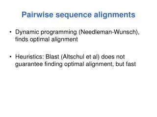
Sequence alignment techniques are crucial in bioinformatics for understanding evolutionary relationships among genes and proteins. This guide covers the basics of dot plots, simple alignments, scoring matrices, and dynamic programming, specifically the Needleman-Wunsch algorithm. It explains how these methods enable researchers to analyze similarities and differences in nucleotide or amino acid sequences, facilitating the prediction of functions for new genetic sequences and insights into their evolutionary histories.

Fundamentals of Sequence Alignment in Bioinformatics
E N D
Presentation Transcript
Database searchand pairwise alignments “It is a capital mistake to theorize before one has data. Insensibly one begins to twist facts to suit theories, instead of theories to suit facts.” (A. Conan Doyle, A scandal in Bohemia, Strand Magazine, July 1891)
Table of contents • Dot plots • Simple alignments • Gap • Score matrices • Dynamic programming: The Needleman-Wunsch algorithm • Global and local alignments • Database search • Multiple sequence alignments
Introduction 1 • Each alignment among two or more nucleotide or amino acid sequences is an explicit assumption about their common evolutionary history • Comparisons among related sequences have facilitated many advances in understanding their information content and their function • Techniques for sequence alignment and sequence comparison, and similarity search algorithms in biological databases are fundamental in Bioinformatics
Introduction 2 • Sequences closely related to each other are usually easy to align and, conversely, the quality of an alignment is an important indicator of their level of correlation • Sequence alignments are used to: • determine the function of a newly discovered genetic sequence (comparison with similar sequences) • determine the evolutionary relationships between genes, proteins, and entire species • predict the structure and the function of new proteins based on known “similar” proteins
Dot plots 1 • Probably, the simplest method to reveal analogies between two sequences consists in displaying the similarity regions using dot plots • The dot plot is a graphical method to display similarity • Less intuitive is its close relationship with the alignments • The dot plot is represented by a table or a matrix or, alternatively, in a Cartesian plane • The lines or the xaxis correspond to the residues of a sequence, and the columns or the yaxis to the residues of the other
Dot plots 2 (a) (b) Dot plots: (a) matrix representation and (b) graphical representation in the Cartesian plane
Dot plots 3 • The similarity regions will thus be viewed as diagonal lines, that proceed from SouthWest to NorthEast; repeated sequences will produce parallel diagonals • Therefore, dot plots capture, in a single image, not only the overall similarity between two sequences, but also the complete set and the relative quality of the different possible alignments • Often, some similarity may be shifted, so as to appear on parallel, but not collinear, diagonals • This indicates the presence of insertion/deletion phenomena occurred in the segments between the similarity regions
Dot plots 4 • In the dot plot matrices, random identities produce a high background noise (especially for long sequences) • This happens almost always in the alignments between nucleic acids, due to the alphabet composed by only four letters • To reduce the noise, short sequences (in sliding windows) should be compared instead of single nucleotids • In this case, the dot is reported only when sresidues coincide within a window of dimension w
Dot plots 5 • Increasing s values corresponds to increase the requested precision (maximum for s = w) • Obviously, the variation of w and s has a significant influence on the background noise • The best experimental values for w and s, with respect to nucleotide and protein sequences, are empirically determined by atrialanderror process
Dot plots 6 • A dot plot matrix, that actually considers only identities, does not provide a true indication of the similarity relations between proteins, since the nonidentity among amino acids can have very different biological implications • In fact: • In some cases the replacement of a residue with a different one, but with very similar properties (e.g.: leucine and isoleucine), can be almost irrelevant • In other cases, two nonidentical residues can have very different properties
Simple alignments 1 • A simple alignment between two sequences consists in matching pairs of characters belonging to the two sequences • The alignment of nucleotide or aminoacid sequences reflects their evolutionary relationship, namely their homology, i.e. the presence of a common ancestor • A score for homology does not exist: at any given position of an alignment, the two sequences may share an ancestor or not • The overall similarity can instead be quantified by means of a fractional value
Simple alignments 2 • In particular, in any given position within a sequence, three types of changes may occur: • A mutation that replaces one character with another • An insertion, which adds one or more characters • A deletion, which eliminates one or more characters • In Nature, insertions and deletions are significantly less frequent than mutations • Since there are no homologues of nucleotides inserted or deleted, gaps are commonly added in the alignments, in order to reflect the occurrence of this type of changes
Simple alignments 3 • In the simplest case, in which gaps are not allowed, the alignment of two sequences is reduced to the choice of the starting point for the shorter sequence AATCTATA AATCTATA AATCTATA AAGATA AAGATA AAGATA • To determine which of the three alignments is “optimal”, it is necessary to establish a score to comparatively evaluate each alignment where nis the length of the longest sequence • For a score of nomatching/matching equal to 0/1, the three alignments are evaluated respectively 4, 1 and 3 { n Correspondence score, if seq1iseq2i Noncorrespondence score, if seq1iseq2i i1
Gaps • Considering the possibility that insertion and deletion events can occur, significantly increases the number of possible alignments between pairs of sequences • For example, the two sequences AATCTATA and AAGATA that can be aligned without gaps in only three ways, admit 28 different alignments, with the insertion of two gaps within the shorter sequence • Example AATCTATA AATCTATA AATCTATA AAGATA AAGATA AAGATA
Simple penalties for gaps’ insertion • Introduction, in the alignment evaluation score, of a penalty term for a gap insertion (gap penalty) • Assuming a score of nomatching/matching equal to 0/1 and a gap penalty equal to 1, the scores for the three alignments with gaps would be 1, 3, 3 AATCTATA AATCTATA AATCTATA AAGATA AAGATA AAGATA Penalty for a gap insertion, if seq1i“” o seq2i “” { n Correspondence score, if seq1iseq2i i1 Noncorrespondence score, ifseq1iseq2i
Penalties for the presence and the length of a gap 1 • Using a simple gap penalty, it is common to evidence many “optimal” alignments (depending on the chosen criterion) • Choose different penalty values for single gaps and gaps that appear in sequence • Concretely, any pairwise alignment represents a hypothesis about the evolutionary path that the two sequences have undertaken from the last common ancestor • When considering several competing hypotheses, the one that invokes the fewest number of improbable events is, by definition, the most probably correct
Penalties for the presence and the length of a gap 2 • Let s1 and s2 be two arbitrary DNA sequences of length 12 and 9, respectively • Each alignment will necessarily have three gaps in the shorter sequence • Assuming that s1 and s2 are homologous sequences, the difference in length can be caused by the insertion of nucleotides in the longer sequence, or by the deletion of nucleotides in the shorter sequence, or by a combination of the two events • Since the sequence of the ancestor is unknown, no methods exist able to determine the cause of a gap, which is attributed generally to an indel event (insertion/deletion) • Moreover, since multiple insertions/deletions are not uncommon, it is statistically more likely that the difference in length between the two sequences was due to a single indel of 3 nucleotides, rather than to many distinct indels
Penalties for the presence and the length of a gap 3 • The scoring function has to reward alignments that are most likely from the evolutionary point of view • By assigning a penalty on the length of the gap (which depends on the number of sequential characters missed) lower than the penalty for the creation of new gaps, the scoring function rewards the alignments that have sequential gaps • Example: using a gap creation penalty equal to 2, a length penalty of 1 (for each gap), and nomatching/ matching values equal to 0/1, the scores in the three cases below are respectively 3, 1, 1 AATCTATA AATCTATA AATCTATA AAGATA AAGATA AAGATA
Score matrices 1 • Just as the gap penalty, that can be adapted to reward alignments evolutionarily more plausible, so the nomatching penalty can be made nonuniform, based on the simple observation that some substitutions are more common than others • Example: let us consider two protein sequences, one of which has an alanine at a given position • A substitution with another amino acid small and hydrophobic, such as valine, has a lower impact on the resulting protein with respect to a replacement with a large and charged residue such as, for example, lysine
Score matrices 2 Alanine Valine Lysine
Score matrices 3 Nucleotides’ matches are moderately rewarded, while a small penalty is given to transition events (substitution between purines/pyrimidines,A-G/C-T); instead, a more severe penalty is assigned for transversions, in which a purine replaces a pyrimidine or vice versa • Intuitively, a conservative substitution, unlike a more drastic one, may occur more frequently, because it preserves the original functionality of the protein • Given an alignment score for each possible pair of nucleotides or residues, the score matrix is used to assign a value to each position of an alignment, except gaps • Example
Score matrices 4 • Several criteria can be considered in setting up a scoring matrix for amino acid sequence alignments • Physicochemical similarity • Observed replacement frequencies • In similarity based matrices, the coupling of two different amino acids, which, however, have both functional aromatic groups (hydrophobic amino acids, characterized by a side chain containing a benzene ring, such as phenylalanine, tyrosine and tryptophan) could receive a positive score, while the coupling of nonpolar with charged amino acids could be penalized
Score matrices 5 • Score matrices can be derived according to the hydrophobicity, the presence of charge, the electronegativity, and the size of the particular residue • Alternatively, similarity criteria based on the encoding genome can also be used: the assigned score is proportional to the minimum number of nucleotide substitutions necessary to convert a codon to another • Difficulty in combining, in a single “significant” matrix, chemical, physical and genetic scores
Score matrices 6 • The most common method to derive score matrices consists in observing the actual frequencies of amino acid substitutions in Nature • If a replacement which involves two particular amino acids is frequently observed, their alignment obtains a favorable score • Vice versa, alignments between residues which, during evolution, are rarely observed must be penalized
PAM matrices 1 • PAM matrices exploit the concept of Point (or Percent)Accepted Mutation; they were proposed in 1978, by M. Dayhoffet al., on the basis of a study on molecular phylogeny involving 71 protein families • PAM matrices were developed by examining mutations within superfamilies of closely related proteins, also noting how observed substitutions did not happen at random • Some amino acid substitutions occur more frequently than others, probably because they do not significantly alter the structure and the function of a protein • Homologous proteins need not to be necessarily constituted by the same amino acids in each position
PAM matrices 2 • Two proteins are “distant” 1 unit PAM if they differ for a single amino acid out of 100, and if the mutation is accepted, i.e. it does not result in a loss of functionality • In other words… two sequences s1 and s2are distant 1 unit PAM if s1can be transformed into s2with a point mutation per 100 amino acids, on average • Since the amino acid at a certain position may change several times and then may return to the original character, the two sequences that are 1 PAM may differ by less than 1%
PAM matrices 3 • Examples of this type of protein families collect orthologous proteins (which perform the same function in different organisms); instead, pathological changes, that are associated to loss of functionality, do not belong to this class • To generate a PAM 1 matrix, we consider a pair (or more) of very similar protein sequences (with an identity 85%), for which the alignment can be defined without ambiguity
PAM matrices 4 • Based on this set of proteins, a PAM 1 score matrix can be defined as follows: • Calculation of an alignment among sequences with very high identity • For each pair of amino acids i and j, calculation of Fij, the number of times that the amino acid j is replaced by i • For each amino acid j, evaluation of the relative mutability nj (the number of substitution of such amino acid, appropriately normalized) • Evaluation of Mij, the mutation probability for each amino acid pair ji • Finally, each PAM 1 element, Pij, is evaluated by applying the logarithm to Mij, previously normalized w.r.t. the frequency of the residue i (PAM 1 is also called the logodds matrix)
PAM matrices 5 • Example (to be continued) • Construction of a multiple sequence alignment: ACGCTAFKI GCGCTLFKI GCGCTAFKI ASGCTAFKL ACGCTAFKL ACACTAFKL GCGCTGFKI
PAM matrices 6 • Example (to be continued) • A phylogenetic tree is created, that indicates the order in which substitutions may have been occurred during evolution ACGCTAFKI AG IL GCGCTAFKI ACGCTAFKL AL AG GA CS GCGCTGFKI GCGCTLFKI ASGCTAFKL ACACTAFKL
PAM matrices 7 • Example (to be continued) • For each amino acid, we calculate the frequency of replacement (with any other amino acid) • It is assumed that the substitutions are symmetric, that is they occur with the same probability with respect to a given pair of amino acids • For instance, in order to determine the substitution frequency between A and G, FG,AFA,G, we count all the branches AG and GA • FG,A 3
PAM matrices 8 • Example (to be continued) • Calculation of the relative mutability njof each amino acid • The mutability mjis the number of times an amino acid is replaced by any other in the phylogenetic tree • This number is then normalized by the total number of mutations that may have some effects on the residue • ...that is, the denominator of the fraction is given by the total number of substitutions in the tree, multiplied by two, multiplied by the frequency of the particular amino acid, multiplied by a scale factor equal to 100 • The scale factor 100 is used because the PAM 1 matrix represents the substitution probability per 100 residues
PAM matrices 9 • Example (to be continued) • Let us consider the amino acid A(alanine): there are 4 mutations involving A in the phylogenetic tree (mA 4) • This value must be divided by twice the total number of mutations (6212), multiplied by the relative frequency of the residue fA (10630.159), multiplied by 100 • nA4(120.159100)0.0209
PAM matrices 10 • Example (to be continued) • Let us calculate the mutation probability Mij, for each pair of amino acids • MijnjFij/jFij • and then… • MG,A(0.02093)40.0156 • where the denominator jFij represents the total number of substitutions that involves A in the phylogenetic tree
PAM matrices 11 • Example • Finally, each Mijmust be divided by the frequency of the residue i; the logarithm of the resulting value constitutes the corresponding element of the PAM matrix, Pij • For G, the frequency fGis equal to 0.159 (1063) • For G and A, PG,Alog(0.01560.159)1.01 • By repeating the above procedure for each pair of amino acids we can obtain all the extradiagonal values of the PAM matrix, whereasPiiare calculated posing Mii1niand executing 6)
PAM matrices 12 • Higher order PAM matrices are generated by successive multiplications of the PAM 1 matrix, since the probability of two independent events is equal to the product of the probabilities of each individual event • While for the PAM 1 matrix it holds that a mutational event corresponds to a difference of 1%, this is not true for higher order PAM matrices • Indeed, subsequent mutations have a gradually increasing chance to happen in correspondence of already mutated amino acids • The degree of difference increases with the increase in the number of mutations, but while it can tend to infinity, the difference tends asymptotically to 100%
PAM matrices 13 • The choice of the most suitable PAM matrix with respect to a particular alignment of sequences, depends on their length and on their correlation degree • PAM 2 is calculated from PAM 1 assuming another evolutionary step • PAM n is obtained from PAM n1 • PAM 100, therefore, represents 100 evolutionary steps, in each of which there was a 1% of substitutions compared to the previous step phylogenetically close sequences phylogenetically distant sequences PAM 1 PAM 100 PAM 250
PAM matrices 14 PAM 250 matrix
PAM matrices 15 • It is worth noting that: • Each PAM matrix element Pijdescribes how much the substitution of the amino acid Aj with the amino acid Ai is more (or less) frequent that a random mutation • Therefore: • Pij 0 more frequent than a random mutation • Pij 0 frequent as a random mutation • Pij0 less frequent than a random mutation
BLOSUM matrices 1 The BLOSUM matrices (BLOcks amino acid SUbstitution Matrices) were introduced in 1992 by S. Henikoff and J. G. Henikoff to assign a score to substitutions between amino acid sequences Their purpose was to replace the PAM matrices, making use of the increased amount of data that had become available after the work of Dayhoff The BLOCKS database contains multiply aligned ungapped segments corresponding to the most highly conserved regions of proteins (local alignment versus global alignment) To get the BLOSUM matrices, related proteins are grouped, using statistical techniques, like clustering 40
BLOSUM matrices 2 The clustering approach helps to eliminate problems that can occur when there is a very low replacement frequency for a specific pair of amino acids Each alignments’ group contains sequences with a number of identical amino acids grater than a certain percentage N For example, in the construction of the BLOSUM62 matrix, each cluster will consist of sequences that have more than 62% identity From each block, it is possible to derive the relative frequency of amino acid replacements, which can be used to calculate a score matrix 41
BLOSUM matrices 3 The elements of the BLOSUM matrix, Bij, are evaluated based on the following relation Bij = klog(M(Ai,Aj)/C(Ai,Aj)),kcostant M(Ai,Aj) is the substitution frequency of the amino acid Ai with the amino acid Aj, observed in the groups of the considered homologous proteins C(Ai,Aj)is the expected substitution frequency, represented by the product of the frequencies of amino acids AjandAj in all the groups of the considered homologous proteins Even in this case, the matrix element (i,j) is proportional to the substitution frequency of the amino acid Aiwith the amino acid Aj phylogenetically distant sequences phylogenetically close sequences 42 BLOSUM35 BLOSUM62
PAM or BLOSUM 1 The two types of matrices start from different assumptions For PAM matrices, it is assumed that the observed amino acid substitutions for large evolutionary distances derive solely by the summing of many independent mutations; the resulting scores express how likely it is that the pairing of a particular couple of amino acids is due to homology rather than to randomness The BLOSUM matrices are not explicitly based on an evolutionary model of mutations; each block is obtained from the direct observation of a family of related proteins (so probably also evolutionarily related), but without explicitly evaluate their similarity 44
PAM or BLOSUM 2 An increasing PAM index describes a suitable score for “distant” proteins, expressing also an evolutionary distance; instead, an increasing BLOSUM index represents a suitable score for protein similar to each others, expressing the minimum conservation value for the BLOCK PAM matrices tend to reward amino acid substitutions resulting from single base mutations, also penalizing substitutions involving more complex changes in the codons; instead, they do not reward structural amino acid motifs, as the BLOSUMs do 45
PAM or BLOSUM 3 The comparison between PAM and BLOSUM, to a comparable level of substitutions, indicates that the two types of matrices produce similar results Typically, the BLOSUM matrices are deemed most suitable to search for sequence similarity The BLOSUM62 matrix is normally set as the default in the similarity search software In any case, it is important to choose the most suitable matrix based on the phylogenetic distance between the sequences to be compared For phylogenetically close sequences (and organisms) low index PAM or high index BLOSUM must be chosen For phylogenetically distant sequences, high index PAM or low index BLOSUM are suitable 46
Dynamic Programming:TheNeedleman-Wunsch algorithm 1 Once having selected a method for assigning a score to an alignment, it is necessary to define an algorithm to determine the best alignment(s) between two sequences The exhaustive search among all possible alignments is generally impractical For two sequences, respectively 100 and 95 nucleotides long, there are 55 million possible alignments, just only in the case of five gaps inserted in the shorter sequence The exhaustive search approach becomes rapidly intractable Using dynamic programming, the problem can be divided into subproblems of more “reasonable” size, whose solutions must be recombined to form the solution of the original problem 47
S. B. Needleman and C. D. Wunsch, in 1970, were the first who solved this problem with an algorithm able to find global similarities, in a time proportional to the product of the lengths of the two sequences The key for understanding this approach is to observe how the alignment problem can be divided into subproblems Dynamic Programming:TheNeedleman-Wunsch algorithm 2 48
Dynamic Programming:TheNeedleman-Wunsch algorithm 3 • Example(to be continued) AlignCACGA and CGA with the assumption of uniformly penalizing gaps and mismatches • Possible choices to be made with respect to the first character: • Place a gap in the first place of the first sequence (counterintuitive, given that the first sequence is longer) • Place a gap in the first place of the second sequence • Align the first two characters • In the first two cases, the alignment score for the first position will be equal to the gap penalty • In the third case, the alignment score for the first position will be equal to the match score • The rest of the score will depend, in all the cases, on the way in which the remaining part of the two sequences will be aligned 49
Dynamic Programming:TheNeedleman-Wunsch algorithm 4 • Example (to be continued) • If we knew the score for the best alignment between the remaining parts of the sequences, we could easily calculate the best overall score relative to the three possible choices 50