Download
1 / 47
490 likes | 830 Vues
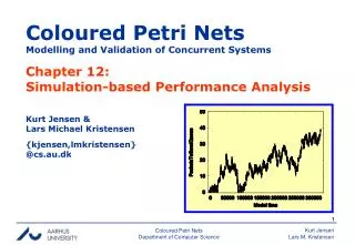
Chapter 12: Simulation-based Performance Analysis. Coloured Petri Nets Modelling and Validation of Concurrent Systems. Kurt Jensen & Lars Michael Kristensen {kjensen,lmkristensen} @cs.au.dk. Performance analysis.

E N D
Chapter 12: Simulation-based Performance Analysis Coloured Petri NetsModelling and Validation of Concurrent Systems Kurt Jensen &Lars Michael Kristensen {kjensen,lmkristensen}@cs.au.dk Coloured Petri Nets Department of Computer Science
Performance analysis • Performance analysis is a central issue in the development and configuration of concurrent systems: • Evaluate existing or planned systems. • Compare alternative implementations of a system. • Search for optimal configuration(s) of a system. • Performance measures of interests include average queue lengths, average delay, throughput, and resource utilisation. • Performance analysis of timed CPN models is done by automaticsimulations. • To estimateperformance measures, numerical data is collected from the occurring binding elements and markings reached. • To get reliable results the simulations must be lengthy or repeated a number of times (e.g. with different parameters). Coloured Petri Nets Department of Computer Science
Timed protocol for performance analysis • To be able to estimate performance measures we make a few modifications of the timed CPN model for the protocol. • We now have a hierarchical model with three modules: • Overview. • Generation of packets to be transmitted (workload). • Protocol to transmit packets and acknowledgments. Coloured Petri Nets Department of Computer Science
Generation of data packets colset NO = int timed; var n : NO; Used to recordTime Of Arrival colset DATA = string timed; colset TOA = int; (* Time Of Arrival *) colset DATAPACKET = product NO * DATA * TOA timed; fun NextArrival() = discrete(200,220); Uniform discrete distribution fun NewDataPacket n = (n, "p"^NO.mkstr(n)^" ", ModelTime()); Returns value of global clock Coloured Petri Nets Department of Computer Science
Data packet arrival • Next data packet will arrive at time 657 = 439 + 218. (DataPacketArrives, <n=3>) 439 Next packet NextArrival() = 218 New packet Coloured Petri Nets Department of Computer Science
Protocol module More fine-grained modelling of success rate Data packets are removed when they are acknowledged val successrate = 0.9; fun Success () = uniform(0.0,1.0) <= successrate; Uniform continuous distribution Coloured Petri Nets Department of Computer Science
Data collection monitors • Data collection in CPN Tools is done by data collection monitors. • They extract numerical data from occurring binding elements and the markings reached in a simulation. • The monitors are defined by means of four monitor functions: • Predicate function determines when data is collected. • Observation function determines what data is collected. • Start function (optional) collects data from the initial marking. • Stop function (optional) collects data from the final marking. M0 M M’ Mfinal (t,b) start(M0) if pred((t,b),M’)then obs((t,b),M’) stop(Mfinal) Coloured Petri Nets Department of Computer Science
Monitor functions • Monitor functions are implemented in CPN ML and consist typically of 5-10 lines of code. • CPN Tools: • supports a set of standard data collection monitors for which the monitor functions are generated automatically. • generates template code for user-defined data collection monitors –which can then be adapted by the user. • A monitor has an associated set of places andtransitions determining what can be referred to in monitor functions. • This is exploited by CPN Tools to reduce the number of times monitor functions are invoked. Coloured Petri Nets Department of Computer Science
Data packets reception monitor • Calculates the number of data packets being received by the receiver, i.e. the number of occurrences of the ReceivePacket. • Implemented by a standard data collection monitor: CountTransitionOccurrences. • The user only needs to selectthe transition. • Not necessary to write any code. • A counter within the monitorholds the number ofoccurrences. Coloured Petri Nets Department of Computer Science
Duplicate receptions monitor • Calculates the number of duplicate data packets received, i.e. the number of occurrences of ReceivePacket with a binding where n<>k. • A user-defined data collection monitor is required since the property is model-specific. • Predicate function: fun pred (Protocol’Receive_Packet (1,{d,data,k,n,t})) = true | pred _ = false; • Observation function: fun obs (Protocol’Receive_Packet (1,{d,data,k,n,t})) = if n<>k then 1 else 0 | obs _ = 0; Coloured Petri Nets Department of Computer Science
Data packet delay monitor • Calculates the delay from a data packet arrives onPacketsToSend until it is received on DataReceived. • Uses the time of arrival field in the data packets. colset DATAPACKET = product NO * DATA * TOA timed; var t : TOA; (* Time Of Arrival *) • Predicate function: fun pred (Protocol’Receive_Packet (1,{d,data,k,n,t})) = n=k | pred _ = false • Observation function: fun obs (Protocol’Receive_Packet (1, {d,data,k,n,t})) = ModelTime()-t+17 | obs _ = 0 Coloured Petri Nets Department of Computer Science
PacketsToSend queue monitor • Calculates the average number of data packets in queue at the sender, i.e. the number of tokens on PacketsToSend. • Implemented by a standard datacollection monitor: MarkingSize. • The user only needs to selectthe place. • Not necessary to write any code. • The monitor takes into account the amount of time that tokens are present on the place. Coloured Petri Nets Department of Computer Science
Example simulation Step Time Binding element Tokens 0 0 – 0 1 0 (DataPacketArrives, n=1) 1 2 0 (SendPacket, n=1, d="p1", t=0) 1 3 9 (TransmitPacket, n=1,d="p1", t=0) 1 4 184 (SendPacket, n=1, d="p1", t=0) 1 5 193 (TransmitPacket, n=1, d="p1", t=0) 1 6 216 (DataPacketArrives, n=2) 2 7 231 (ReceivePacket, n=1, d="p1", t=0, data="",k=1) 2 8 248 (TransmitAck, n=2, t=0) 2 9 276 (ReceiveAck, n=2, t=0,k=2) 2 10 283 (SendPacket, n=2,d="p2 ",t=436) 2 11 283 (RemovePacket, n=1, t=0,d="p1 ") 1 12 292 (TransmitPacket, n=2,d="p2 ", t=216) 1 13 347 (ReceivePacket, n=2,k=2,d="p2 ",t=216, data="p1 ") 1 Coloured Petri Nets Department of Computer Science
i=1 xi n 0+1+1+1+1+1+2+2+2+2+2+1+1+1 avrg = n = 1.29 14 Discrete-parameters statistics • Average number of tokens: Coloured Petri Nets Department of Computer Science
sumt = (i=1 xi(ti+1– ti))+xn(t – tn) n–1 sumt avrgt = t – t1 avrg347 = 414/347 = 1.19 0x0 + 1x0 + 1x9 + 1x175 + 1x9 + 1x23 + 2x15 + 2x17 + 2x28 + 2x7 + 2x0 + 1x9 + 1x55 + 1x0 = 414 1.29 Continuous-time statistics • Time-average number of tokens: Time of calculation The individual values are weighted with their duration Untimed average Coloured Petri Nets Department of Computer Science
Network buffer queue monitor • Calculates the average number of data packets and acknowledgements on the network, i.e. the number of tokens on the places B and D: • Implemented by a user-defined data collection monitor. Coloured Petri Nets Department of Computer Science
Network buffer queue monitor • Predicate function returns true whenever one of the transitions TransmitPacket, ReceivePacket, TransmitAck or ReceiveAck occurs. • Observation function: fun obs (bindelem, Protocol’B_1_mark : DATAPACKET tms, Protocol’D_1_mark : ACK tms) = (size Protocol’B_1_mark) + (size Protocol’D_1_mark); • We also need to make an observation at the simulation start. • Start function: fun start (Protocol’B_1_mark : DATAPACKET tms, Protocol’D_1_mark : ACK tms) = SOME ((size Protocol’B_1_mark) + (size Protocol’D_1_mark)); Data collection in initial marking is optional Coloured Petri Nets Department of Computer Science
Throughput monitor • Calculates the number of non-duplicate data packets delivered by the protocol per time unit. Number of observations Existing monitor (makes an observation for each received non-duplicate packet) • Stop function: fun stop () = let val received = Real.fromInt (DataPacketDelay.count()); val modeltime = Real.fromInt (ModelTime()); in SOME (received / modeltime) end; Data collection at the end of the simulation is optional Coloured Petri Nets Department of Computer Science
Last occurrence of ReceivePacket Simulation stopped model time 17 excess time Receiver utilisation monitor • Calculates the proportion of time that the receiver is busy processing packets. • Can be computed by considering the number of occurrencesof the ReceivePacket transition which each takes 17 units of model time. • Simulation may have been stopped before the last receive operation has ended. Coloured Petri Nets Department of Computer Science
Receiver utilisation monitor Existing monitor (makes an observation for each received packet) Number of observations • Stop function: fun stop (Protocol’NextRec_1_mark : NO tms) = let val busytime = DataPacketReceptions.count() * 17; val ts = timestamp (Protocol’NextRec_1_mark); val excesstime = Int.max (ts – ModelTime(),0); val busytime’ = Real.fromInt (busytime – excesstime); in SOME (busytime’/(Real.fromInt (Modeltime()))) end; End of last occurrence of ReceivePacket Coloured Petri Nets Department of Computer Science
Simulation output • System parameters: val successrate = 0.9; fun NextArrival() = discrete(200,220); fun Delay() = discrete(25,75); val Wait = 175; • Log file for PacketsToSendQueue monitor: #data counter step time 0 1 0 0 1 2 1 0 1 3 2 0 1 4 4 184 2 5 6 216 2 6 10 283 1 7 11 283 Coloured Petri Nets Department of Computer Science
Log files can be post-processed • Data collection log files can be imported into a spreadsheet or plotted. • CPN Tools generates scripts for plotting log files using gnuplot. • Easy to create a number of different kinds of graphs. Coloured Petri Nets Department of Computer Science
Statistics from simulations • Monitors make repeated observations of numerical values, such as packet delay, reception of duplicate data packets, or the number of tokens on a place. • The individual observations are often of little interest, but it is interesting to calculate statistics for the total set of observations: • It is not interesting to know the packet delay of a single data packet. • But it is interesting to know the average and maximum packet delay for the entire set of the data packets. • A statistic is a quantity, such as the average or maximum, that is computed from an observed data set. Coloured Petri Nets Department of Computer Science
Discrete-parameter / continuous-time • A monitor calculates either: • the regular average or • the time-average for the data values it collects. • A monitor that calculates the (regular) average is said to calculate discrete-parameter statistics. • A monitor that calculates time-average is said to calculate continuous-time statistics. • An option for the monitor determines which kind of statistics it calculates. Coloured Petri Nets Department of Computer Science
Statistics from monitors • Monitorscalculate a number of different statistics such as: • count (number of observations), • minimum and maximum value, • sum, • average, • first and last (i.e. most recent) value observed. • Continuous-time monitors also calculate: • time of first and last observation, • interval of time since first observation. • Statistics are accessed by a set of predefined functionssuch as count, sum, avrg, and max. • DataPacketDelay.count() – used in the Throughput monitor. Coloured Petri Nets Department of Computer Science
Monitor Count Average StD Min Max PacketsToSendQueue 4,219 1.2583 0.9207 0 5 NetworkBufferQueue 5,784 0.5004 0.5000 0 1 Monitor Count Sum Average StD Min Max DataPacketDelay 1,309 243,873 186.30 152.89 51 851 DataPacketReceptions 1,439 1,439 1.0 0.0 1 1 DuplicateReceptions 1,439 130 0.0903 0.2868 0 1 Throughput 1 0.0048 0.0048 0.0 0.0048 0.0048 ReceiverUtilization 1 0.0889 0.0889 0.0 0.0889 0.0889 Simulation performance report • Contains statistics calculated during a single simulation: • Length of simulation: 275,201 time units and 10,000 steps. • Continuous-time statistics: • Discrete-parameter statistics: Coloured Petri Nets Department of Computer Science
Performance Measure 1 2 3 4 5 PacketsToSendQueue 1.57021.2567 1.3853 1.2824 1.2762 NetworkBufferQueue 0.5047 0.4946 0.5093 0.5125 0.5073 DataPacketDelay 250.95184.34 210.20 191.93 189.07 DuplicateReceptions 0.1026 0.09380.1137 0.0983 0.1073 Throughput 0.0047680.004758 0.004766 0.004763 0.004760 ReceiverUtilisation 0.089749 0.088802 0.0905700.088693 0.089821 Simulation experiments • Most simulation models contain random behaviour. • Simulation output data also exhibits random behaviour. • Different simulations will result in different estimates. • Care must be taken when interpreting and analysing the output data. • Average of monitors calculated for five different simulations: Coloured Petri Nets Department of Computer Science
Confidence intervals • Standard technique for determining how reliable estimates are. • A 95% confidence intervalis an interval which is determined such that there is a 95% likelihood that the true value of the performance measure is within the interval. • The most frequently used confidence intervals are confidence intervals for averages of estimates of performance measures. • CPN Tools can automatically compute confidence intervals and save these in performance report files. Coloured Petri Nets Department of Computer Science
Confidence intervals for DataPacketDelay • 90%, 95% and 99%. • Number of simulations (95%). Coloured Petri Nets Department of Computer Science
Simulation replications • We want to calculate estimates of performance measures from a set of independent, statistically identical simulations: • Start and stop in the same way (e.g. when 1,500 unique data packets have been received). • Same system parameters (e.g., the time between data packet arrivals). Replications.run 5; Run five simulations and gather statistics from them Predefined function Coloured Petri Nets Department of Computer Science
Packets received monitor • Simulations can be stopped by a breakpoint monitor. • Stops the simulation when the predicate functionevaluates to true. • We may e.g. want to stop when 1,500 unique data packets have been received. fun pred (Protocol’Receive_Packet (1, {k,...})) = k > 1500 | pred _ = false; Coloured Petri Nets Department of Computer Science
Simulation replication report Simulation no.: 1 Steps.........: 11,530 Model time....: 314,810 Stop reason...: The following stop criteria are fulfilled: - Breakpoint: PacketsReceived Time to run simulation: 2 seconds Simulation no.: 2 Steps.........: 11,450 Model time....: 315,488 Stop reason...: The following stop criteria are fulfilled: - Breakpoint: PacketsReceived Time to run simulation: 3 seconds Simulation no.: 3 ...... Coloured Petri Nets Department of Computer Science
Monitor Average 95 % StD Min Max PacketsToSendQueue 1.3542 0.1025 0.1169 1.2567 1.5702 NetworkBufferQueue 0.5057 0.0053 0.0061 0.4946 0.5125 DataPacketDelay 205.30 21.43 24.45 184.34 250.95 Performance report from a set ofrepeated simulations • Combines the results from a set of repeated simulations (with the same system parameters). This allows us to: • get more precise results, • estimate the precision of our results (by calculating confidence intervals). Confidence interval Standard deviation Coloured Petri Nets Department of Computer Science
System parameters • The performance of a modelled system is often dependent on a number of parameters. • Simulation-based performance analysis may be used to compare different scenarios or configurations of the system. • In some studies, the scenarios are given, and the purpose of the study is to compare the given configurations and determine the best of these configurations. • If the scenarios are not predetermined, one goal of the simulation study may be to locate the parameters that have the most impact on a particular performance measure. Coloured Petri Nets Department of Computer Science
How to change parameters? • Simulation parameters are typically defined by symbolic constants and functions, e.g.: val successrate = 0.9; fun Success() = uniform(0.0,1.0) <= successrate; • The parameter can be changed by modifying the declaration of the symbolic constant successrate. • In CPN Tools, these changes must be done manually. • The declaration and those parts of the model that depend upon it are rechecked and new code generated for them. Coloured Petri Nets Department of Computer Science
Reference variables • To avoid manual changes and time-consuming rechecks and code generation, we use reference variables to hold parameter values: globref successrate = 90; globref packetarrival = (200,220); globref packetdelay = (25,75); globref retransmitwait = 175; • The keyword globref specifies that a global reference variable is being declared that can be accessed from any part of the CPN model. Coloured Petri Nets Department of Computer Science
Manipulation of reference variables • The values of the reference variables can be accessed by means of the ! operator: fun Success() = discrete(0,100) <= (!successrate); fun Delay() = discrete(!packetdelay); fun NextArrival() = discrete(!packetarrival); fun Wait() = !retransmitwait; • The values of the reference variables can be changed by means of the := operator: successrate := 75; • It is notnecessary to recheck the syntax of any part of a CPN model when the value of a reference variable is changed. Coloured Petri Nets Department of Computer Science
Modified Protocol module Function instead of symbolic constant Coloured Petri Nets Department of Computer Science
Configurations • Colour set declaration: colset INT = int; colset INTxINT = product INT * INT; colset CONFIG = record successrate : INT * packetarrival : INTxINT * packetdelay : INTxINT * retransmitwait : INT; • Example value: {successrate = 90, packetarrival = (200,220), packetdelay = (25,75) retransmitwait = 175} • Update of reference variables: fun setconfig (config : CONFIG) = (successrate := (#successrate config); packetarrival := (#packetarrival config); packetdelay := (#packetdelay config); retransmitwait := (#retransmitwait config)); Coloured Petri Nets Department of Computer Science
Multiple simulation runs • 30 configurations with retransmitwait{10,20,30,...,300}. Pred-declared function val configs = List.tabulate (30,fn i => {successrate = 90, packetarrival = (200,220), packetdelay = (25,75), retransmitwait = 10+(i*10)}); Number of configurations Function to be used on each element in the list [0,1,2,…29] of length 30 • Run n repeated simulations of config. fun runconfig n config = (setconfig config; Replications.run n); • Five runs of each configuration in configs. List.app (runconfig 5) configs; Coloured Petri Nets Department of Computer Science
Performance results • The CPN simulator conducts the specified set of simulations while saving the simulation output in log files and performance reports as described above. • Based on the log files we can create graphs for the monitors: • Data Packet Delay. • PacketsToSend Queue. • Network Buffer Queue. • Receiver Utilisation. • Throughput. Coloured Petri Nets Department of Computer Science
Data Packet Delay • For small time values we get accurate estimates. • For higher time values the confidence intervalsbecome wider. • The retransmission wait has relatively small effect on the average data packet delay as long as it is below 150 time units. • When the retransmission wait is above 250 time units, large average data packet delays are observed because lost data packets now wait a long time before being retransmitted. Coloured Petri Nets Department of Computer Science
PacketsToSend Queue • The curve (and the confidence intervals) is similar to the curve for DataPacketDelay. • When the retransmission wait becomes high, a queue of data packets starts to build up – contributing to the increased data packet delay observed on the previous graph. • To investigate this we consider a log file from a simulation with retransmission wait equal to 300. Coloured Petri Nets Department of Computer Science
PacketsToSend Queue • Log file from a simulation with retransmission wait equal to 300. • The system has become unstable. • Performance measure estimates must be interpreted with great care. • The average number of tokens will depend on how long the simulation is running and can be made arbitrarily large by making the simulation longer. Coloured Petri Nets Department of Computer Science
Network Buffer Queue • We measure the average number of tokens on places B and D. • For all values, we get accurate estimates. • With a small retransmission wait there are more packets on the network – because the frequent retransmissions introduce more packets to be sent. Coloured Petri Nets Department of Computer Science
Receiver Utilisation • When retransmission wait is above 150 there are very few unnecessary retransmissions of data packets. • Hence, the receiver utilisation no longer decreases. Throughput • When retransmission wait is above 250, throughput decreases and the confidence intervals become large. Coloured Petri Nets Department of Computer Science
Questions Coloured Petri Nets Department of Computer Science