Download

1 / 56
650 likes | 1.74k Vues
Numerical Integration of Partial Differential Equations (PDEs). Introduction to PDEs. Semi-analytic methods to solve PDEs. Introduction to Finite Differences. Stationary Problems, Elliptic PDEs. Time dependent Problems. Complex Problems in Solar System Research. Introduction to PDEs.

E N D
Numerical Integration ofPartial Differential Equations (PDEs) • Introduction to PDEs. • Semi-analytic methods to solve PDEs. • Introduction to Finite Differences. • Stationary Problems, Elliptic PDEs. • Time dependent Problems. • Complex Problems in Solar System Research.
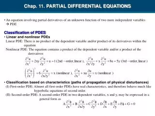
Introduction to PDEs. • Definition of Partial Differential Equations. • Second Order PDEs.-Elliptic-Parabolic-Hyperbolic • Linear, nonlinear and quasi-linear PDEs. • What is a well posed problem? • Boundary value Problems (stationary). • Initial value problems (time dependent).
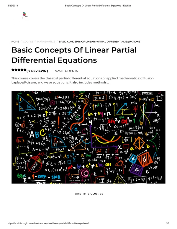
Differential Equations • A differential equation is an equation for an unknown function of one or several variables that relates the values of the function itself and of its derivatives of various orders. • Ordinary Differential Equation:Function has 1 independent variable. • Partial Differential Equation:At least 2 independent variables.
Physical systems are oftendescribed by coupledPartial Differential Equations (PDEs) • Maxwell equations • Navier-Stokes and Euler equationsin fluid dynamics. • MHD-equations in plasma physics • Einstein-equations for general relativity • ... • ...
PDEs definitions • General (implicit) form for one function u(x,y) : • Highest derivative defines order of PDE • Explicit PDE => We can resolve the equationto the highest derivative of u. • Linear PDE => PDE is linear in u(x,y) and for all derivatives of u(x,y) • Semi-linear PDEs are nonlinear PDEs, whichare linear in the highest order derivative.
Linear PDEs of 2. Order • a(x,y)c(x,y) − b(x,y)2 / 4 > 0 Elliptic • a(x,y)c(x,y) − b(x,y)2 / 4 = 0 Parabolic • a(x,y)c(x,y) − b(x,y)2 / 4 < 0 Hyperbolic Quasi-linear: coefficients depend on u and/or first derivative of u, but NOT on second derivatives.
PDEs and Quadratic Equations • Quadratic equations in the form describe cone sections. • a(x,y)c(x,y) − b(x,y)2 / 4 > 0 Ellipse • a(x,y)c(x,y) − b(x,y)2 / 4 = 0 Parabola • a(x,y)c(x,y) − b(x,y)2 / 4 < 0 Hyperbola
With coordinate transformations these equations can be written in the standard forms: Ellipse: Parabola: Hyperbola: Coordinate transformations can be also applied to get rid of the mixed derivatives in PDEs. (For space dependent coefficients this is only possible locally, not globally)
Linear PDEs of 2. Order • Please note: We still speak of linear PDEs, even ifthe coefficients a(x,y) ... e(x,y) might be nonlinearin x and y. • Linearity is required only in the unknown function u and all derivatives of u. • Further simplification are:-constant coefficients a-e,-vanishing mixed derivatives (b=0) -no lower order derivates (d=e=0) -a vanishing function f=0.
Second Order PDEs with more then2 independent variables • Elliptic: All eigenvalues have the same sign. [Laplace-Eq.] • Parabolic: One eigenvalue is zero. [Diffusion-Eq.] • Hyperbolic: One eigenvalue has opposite sign. [Wave-Eq.] • Ultrahyperbolic: More than one positive and negative eigenvalue. Mixed types are possible for non-constant coefficients,appear frequently in science and are often difficult to solve. Classification by eigenvalues of the coefficient matrix:
Elliptic Equations • Occurs mainly for stationary problems. • Solved as boundary value problem. • Solution is smooth if boundary conditions allow. Example: Poisson and Laplace-Equation (f=0)
Parabolic Equations • The vanishing eigenvalue often related to time derivative. • Describes non-stationary processes. • Solved as Initial- and Boundary-value problem. • Discontinuities / sharp gradients smooth out during temporal evolution. Example: Diffusion-Equation, Heat-conduction
Hyperbolic Equations • The opposite sign eigenvalue is often related to the time derivative. • Initial- and Boundary value problem. • Discontinuities / sharp gradients in initialstate remain during temporal evolution. • A typical example is the Wave equation. • With nonlinear terms involved sharp gradients can form during the evolution => Shocks
Well posed problems(as defined by Hadamard 1902)A problem is well posed if: • A solution exists. • The solution is unique. • The solution depends continuously on the data (boundary and/or initial conditions). 1865-1963 Problems which do not fulfill these criteria are ill-posed. Well posed problems have a good chance to be solved numerically with a stable algorithm.
Ill-posed problems • Ill-posed problems play an important rolein some areas, for example for inverse problems like tomography. • Problem needs to be reformulated fornumerical treatment. • => Add additional constraints, for example smoothness of the solution. • Input data need to be regularized / preprocessed.
Ill-conditioned problems • Even well posed problems can be ill-conditioned. • => Small changes (errors,noise) in data leadto large errors in the solution. • Can occur if continuous problems are solvedapproximately on a numerical grid.PDE => algebraic equation in form Ax = b • Condition number of matrix A: are maximal and minimal eigenvalues of A. • Well conditioned problems have a low condition number.
How to solve PDEs? • PDEs are solved together with appropriateBoundary Conditions and/or Initial Conditions. • Boundary value problem-Dirichlet B.C.: Specify u(x,y,...) on boundaries(say at x=0, x=Lx, y=0, y=Ly in a rectangular box)-von Neumann B.C.: Specify normal gradient of u(x,y,...) on boundaries. In principle boundary can be arbitrary shaped. (but difficult to implement in computer codes)
Initial value problem • Boundary values are usually specified onall boundaries of the computational domain. • Initial conditions are specified in the entirecomputational (spatial) domain, but onlyfor the initial time t=0. • Initial conditions as a Cauchy problem:-Specify initial distribution u(x,y,...,t=0) [for parabolic problems like the Heat equation]- Specify u and du/dt for t=0 [for hyperbolic problems like wave equation.]
Cauchy Boundary conditions • Cauchy B.C. impose both Dirichletand Von Neumann B.C. on part ofthe boundary (for PDEs of 2. order). • More general: For PDEs of order n theCauchy problem specifies u and allderivatives of u, up to the order n-1on parts of the boundary. • In physics the Cauchy problem is oftenrelated to temporal evolution problems (initial conditions specified for t=0) Augustin Louis Cauchy 1789-1857
Introduction to PDEsSummary • What is a well posed problem? Solution exists, is unique, continuous on boundary conditions. • Elliptic (Poisson), Parabolic (Diffusion)and Hyperbolic (Wave) PDEs. • PDEs are solved with boundary conditionsand initial conditions. • What are Dirichlet and von Neumannboundary conditions?
Numerical Integration ofPartial Differential Equations (PDEs) • Introduction to PDEs. • Semi-analytic methods to solve PDEs. • Introduction to Finite Differences. • Stationary Problems, Elliptic PDEs. • Time dependent Problems. • Complex Problems in Solar System Research.
Semi-analytic methods to solve PDEs. • From systems of coupled first order PDEs (which are difficult to solve) to uncoupledPDEs of second order. • Example: From Maxwell equationsto wave equation. • (Semi) analytic methods to solve thewave equation by separation of variables. • Exercise: Solve Diffusion equationby separation of variables.
How to obtain uncoupled 2. orderPDEs from physical laws? • Example: From Maxwell equations to wave equations. • Maxwell equations are a coupled system of first order vector PDEs. • Can we reformulate this equationsto a more simple form? • Here we use the electromagnetic potentials,vectorpotential and scalar potential.
Maxwell equations James C. Maxwell 1831-1879
What do we win with wave equations? • Inhomogenous coupled system ofMaxwell reduces to wave equations. • We get 2. order scalar PDEsfor components of electric andmagnetic potentials. • Equation are not coupled and havesame form. • Well known methods exist to solvethese wave equations.
Wave equation • Electric charges and currents on right side ofwave-equation can be computed from other sources: • Moments of electron and ion-distribution inspace-plasma. • The particle-distributions can be derived fromnumerical simulations, e.g. by solving theVlasov equation for each species. • Here we study the wave equation in vacuum forsimplicity.
(Semi-) analytic methods • Example: Homogenous wave equation • Can be solved by any analytic function f(x-ct) and g(x+ct). • As the homogenous wave equation is alinear equation any linear combination off and g is also a solution of the PDE. • This property can be used to specify boundaryand initial conditions. The appropriate coefficientshave to be found often numerically.
Semi-analytic method: Variable separation Show: demo_wave_sep.pro This is an IDL-program to animate the wave-equation
lecture_diffusion_draft.pro Exercise:1D diffusion equation This is a draft IDL-program to solve the diffusion equation by separation of variables. Task: Find separable solutions forDirichlet and von Neumann boundary conditions and implement them.
Semi-analytic methods Summary • Some (mostly) linear PDEs with constantcoefficients can be solved analytically. • One possibility is the method ‘Separation of variables’, which leads toordinary differential equations. • For linear PDEs.: Superposition of different solutions is also a solution of the PDE.
Numerical Integration ofPartial Differential Equations (PDEs) • Introduction to PDEs. • Semi-analytic methods to solve PDEs. • Introduction to Finite Differences. • Stationary Problems, Elliptic PDEs. • Time dependent Problems. • Complex Problems in Solar System Research.
Introduction to Finite Differences. • Remember the definition of the differential quotient. • How to compute the differential quotientwith a finite number of grid points? • First order and higher order approximations. • Central and one-sided finite differences. • Accuracy of methods for smoothand not smooth functions. • Higher order derivatives.
Numerical methods • Most PDEs cannot be solved analytically. • Variable separation works only for somesimple cases and in particular usually notfor inhomogenous and/or nonlinear PDEs. • Numerical methods require that the PDEbecome discretized on a grid. • Finite difference methods are popular/most commonly used in science. They replace differential equation by difference equations) • Engineers (and a growing number ofscientists too) often use Finite Elements.
Finite differences Remember the definition of differential quotient: • How to compute differential quotient numerically? • Just apply the formular above for a finite h. • For simplicity we use an equidistant grid inx=[0,h,2h,3h,......(n-1) h] and evaluate f(x)on the corresponding grid points xi. • Grid resolution h must be sufficient high.Depends strongly on function f(x)!
Accuracy of finite differences We approximate the derivative of f(x)=sin(n x) on a grid x=0 ...2 Pi with 50 (and 500) grid points by df/dx=(f(x+h)-f(x))/h and comparewith the exact solution df/dx= n cos(n x) Average error done by discretisation: 50 grid points: 0.040 500 grid points: 0.004
Accuracy of finite differences We approximate the derivative of f(x)=sin(n x) on a grid x=0 ...2 Pi with 50 (and 500) grid points by df/dx=(f(x+h)-f(x))/h and comparewith the exact solution df/dx= n cos(n x) Average error done by discretisation: 50 grid points: 2.49 500 grid points: 0.256
Higher accuracy methods Can we use more points for higher accuracy?
Higher accuracy: Central differences • df/dx=(f(x+h)-f(x))/hcomputes the derivativeat x+h/2 and not exactly at x. • The alternative formular df/dx=(f(x)-f(x-h))/hhas the same shortcomings. • We introduce central differences:df/dx=(f(x+h)-f(x-h))/(2 h) which providesthe derivative at x. • Central differences are of 2. order accuracyinstead of 1. order for the simpler methodsabove.
How to find higher order formulars? For sufficient smooth functions we describe the function f(x) locally by polynomial of nth order. To do so n+1grid points are required. n defines the order of the scheme. Make a Taylor expansion (Definition ):