Wallet Study
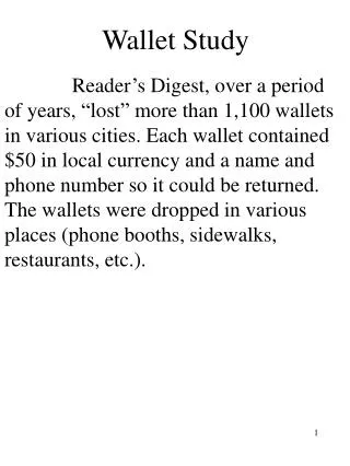
Wallet Study. Reader’s Digest, over a period of years, “lost” more than 1,100 wallets in various cities. Each wallet contained $50 in local currency and a name and phone number so it could be returned. The wallets were dropped in various places (phone booths, sidewalks, restaurants, etc.). .

Wallet Study
E N D
Presentation Transcript
Wallet Study Reader’s Digest, over a period of years, “lost” more than 1,100 wallets in various cities. Each wallet contained $50 in local currency and a name and phone number so it could be returned. The wallets were dropped in various places (phone booths, sidewalks, restaurants, etc.).
Norway 100% Denmark 100% Singapore 90% New Zealand 83% Finland 80% Scotland 80% Australia 70% Japan 70% South Korea 70% Spain 70% Austria 70% Sweden 70% U.S. 67% England 67% India 65% Canada 64% France 60% Brazil 60% Netherlands 60% Thailand 55% Belgium 50% Taiwan 50% Malaysia 50% Germany 45% Portugal 45% Argentina 44% Russia 43% Philippines 40% Wales 40% Italy 35% Switzerland 35% Hong Kong 30% Mexico 21% AVERAGE: 56% Wallets Returned
Wallets ReturnedWallets Kept Seattle 9 1 St. Louis 7 3 Atlanta 5 5 Boston* 7 3 Los Angeles* 6 4 Houston* 5 5 Greensboro, N.C. 7 3 Las Vegas 5 5 Dayton, Ohio 5 5 Concord, N.H. 8 2 Cheyenne, Wyo. 8 2 Meadville, Pa. 8 2 (*wallets dropped in suburbs of these cities) U.S. Cities
Social Outputs Economic outputs depend on social capital, to be sure, but what crime, illegitimacy, loneliness, etc.? Social outputs can also be modelled using production functions. Social outputs can also be assigned dollars values: how much would people pay to increase a social output? The variability in social outputs from differing levels of social capital may be much greater than the variability in economic outputs.
Regressions 1. Specification search (which variables?) 2. Using simple bivariate correlations 3. Weighted regressions 4. Dropping outliers 5. Adding quadratic or log terms for curvature
Available Data pop malework murder cartheft illegit divorce metro retired midage unemp teachsal homeown income bachelor abortion black southern churchm voting
Bivariate Correlations with the Murder Rate malework -.25 cartheft .71 illegit .79 divorce .03 metro .27 retired -.03 midage .14 unemp .38 teachsal .15 homeown -.52 income .23 bachelor .32 abortion .84 black .77 southern .38 churchm .06 voting -.27
Source: Robert Putnam: Bowling Alone, “Selected statistical trend data” http://www.bowlingalone.com/data.php3 (12/8/01)
Correlation Matrix | putnam orgs member trust ---------------------------------------------------- putnam | 1.00 orgs | .81 1.00 member | .73 .58 1.00 trust | .92 .73 .70 1.00
Bivariate Correlations with “putnam” Social Capital malework .58 murder -.74 cartheft -.45 illegit -.56 divorce -.35 metro -.36 retired .15 midage -.05 unemp -.44 teachsal -.13 homeown .05 income .09 bachelor .34 abortion -.30 black -.71 southern -.62 churchm -.02 voting .69
Murder = putnam -2.75 (7.55) R2 = .55 N = 48 Murder = trust -.16 (6.03) R2 = .48 N=41 Murder = orgs -3.44 (5.17) R2 = .35 N=50 Murder = member -1.06 (3.35) R2 = .22 N=40 Murder = putnam orgs trust member -2.60 .08 -.03 .91 (1.89) (0.07) (0.47) (0.71) R2 = .52 N=40 Different Measures
Weighting Murder = putnam income -2.69(7.51) -.00012(1.75) Murder = putnam income -2.48(5.58) -.00014(2.05) (weight = pop) Murder = putnam income -2.46(8.00) -.00018(2.38) (weight = 1/pop) Murder = putnam income -2.69(9.97) -.00012(1.60) (White robust standard errors)
A Regression Murder = .68* Illegit -.25*Homeown (7.78) (2.89)
state v1 1. AL 1.313196 2. AK -.0083414 3. AZ -3.002368 4. AR -.3776368 5. CA .1270525 6. CO 4.011913 7. CT .6871804 8. DE -8.302368 9. DC 20.62919 10. FL -3.582326 11. GA -1.276142 12. HA -4.394481 13. ID 5.293575 14. IL .9854771 15. IN -.028383 16. IA -.3358477 17. KA 2.801039 18. KE .0886737 19. LA -3.010255 20. ME -3.217509 21. MD 1.957757 22. MA .5488002 23. MI .6701256 24. MN 1.619589 25. MS -5.27337 Residuals from Illegit,Homeown 26. MO -.1145223 27. MT -.0974675 28. NE 2.119589 29. NV 1.030039 30. NH 1.85349 31. NJ .9795045 32. NM -5.145649 33. NY -4.276142 34. NC 1.391659 35. ND -1.135848 36. OH -3.414522 37. OK -.6083413 38. OR -.7113263 39. PA -1.172947 40. RI -5.171453 41. SC -3.259298 42. SD -4.209833 43. TN .614687 44. TX 1.582491 45. UT 9.338348 46. VT -1.134354 47. VA 2.237926 48. WA 1.193363 49. WV -1.231369 50. WI .0302502 51. WY 1.387181
1. AL -.87 2. AK . 3. AZ 2.44 4. AR .35 5. CA .83 6. CO .64 7. CT .66 8. DE -2.40 9. DC . 10. FL -.25 11. GA -.58 12. HA . 13. ID -2.94 14. IL 2.70 15. IN 1.76 16. IA -1.22 17. KA 1.26 18. KE -3.59 19. LA 4.01 20. ME -2.42 21. MD 4.29 22. MA -1.98 23. MI 1.78 24. MN .974 25. MS 1.86 Residuals from putnam, income 26. MO 1.85 27. MT 1.40 28. NE .63 29. NV .63 30. NH -1.57 31. NJ -1.60 32. NM 3.75 33. NY -.65 34. NC .18 35. ND -.31 36. OH -2.08 37. OK -.44 38. OR -.26 39. PA -.62 40. RI -3.05 41. SC -.40 42. SD .11 43. TN .13 44. TX -.35 45. UT -1.59 46. VT .28 47. VA .01 48. WA .42 49. WV -4.27 50. WI -.37 51. WY .87
Murder = putnam income -2.69 (7.51) -.00012 (1.75) R2 = .55 Murder = putnam income -2.81 (8.20) -.00016 (2.33) R2 = .63 (WV dropped) Murder = putnam income -2.61 (8.37) -.00016 (2.66) R2 = .65 (WV,MD,LA dropped) Not much happens if outliers are dropped. Dropping Outliers
Murder = illegit homeown -0.68 (7.78) -0.25 (2.89) R2 = .67 Murder = illegit homeown -0.37 (7.31) 0.05 (0.98) R2 = .53 (DC dropped) The effect of illegitimacy becomes smaller, and home ownership becomes insignificant. Dropping Outliers
Murder = illegit homeown -0.68 (7.78) -.25 (2.89) R2 = .67 Murder = log(illegit) homeown 19.20 (5.56) -.33 (3.33) R2 = .55 Murder = illegit illegit2 homeown -1.61 .03 -.07 (6.27) (9.14) (1.23) R2 = .88 Squared and Log Terms
Murder Regression 1 R 2 = .55 Putnam -2.75 (7.55) Regression 2 R 2 = .68 Putnam -1.62 (3.06) Income -0.00028 (2.75) Black 0.15 (3.45) Metro 0.024 (1.18) Southern -1.58 (1.83)
Illegitimacy Regression 1 R 2 = .34 Putnam -4.23 (4.91) Regression 2 R 2 = .50 Putnam -1.82 (1.40) Income -0.00046 (1.81) Black 0.34 (3.16) Metro 0.021 (0.42) Southern -2.79 (1.32)
Male Labor Participation Regression 1 R 2 = .35 Putnam 2.60 (5.08) Regression 2 R 2 = .42 Putnam 2.45 (2.89) Income 0.00012 (0.74) Black 0.007 (0.11) Metro 0.013 (0.42) Southern -0.76 (0.55)
Car Theft Regression 1 R 2 = .21 Putnam -103.86 (3.53) Regression 2 R 2 = .61 Putnam -37.03 (1.04) Income -0.02 (2.92) Black 0.13 (0.04) Metro 8.03 (5.76) Southern -47.85 (2.97)
Aristotle contra Kelvin Kelvin: ``When you measure what you are speaking about and express it in numbers, you know something about it, but when you cannot express it in numbers your knowledge about is of a meagre and unsatisfactory kind.'’ Aristotle: ``...it is the mark of an educated man to look for precision in each class of things just so far as the nature of the subject admits; it is evidently equally foolish to accept probable reasoning from a mathematician and to demand from a rhetorician scientific proofs.'’ Kelvin: ``In science there is only physics; all the rest is stamp collecting.'' Kelvin: ``I can state flatly that heavier than air flying machines are impossible.'’