Download

1 / 28
290 likes | 658 Vues
Software Decision Analysis Techniques Chapters 10-20 in Software Engineering Economics. Economics – The study of how people make decisions in resource-limited situations Macroeconomics Inflation, taxation, balance of payments Microeconomics Make-or-buy, pricing, how much to build

E N D
Software Decision Analysis TechniquesChapters 10-20 in Software Engineering Economics • Economics – The study of how people make decisions in resource-limited situations • Macroeconomics • Inflation, taxation, balance of payments • Microeconomics • Make-or-buy, pricing, how much to build • Software economics decisions • Make-or-buy: Software Product • How many options to build? • Which DP architecture to use? • How much testing (prototyping, specifying) is enough? • How much software to re-use? • Which new features to add first?
Outline of Chapters • 10-12. Context; TPS II Example; Cost-Effectiveness Analysis • Models, optimization, production functions, economies of scale decision criteria • 13-15. Multiple-Goal Decision Analysis I • Net value, marginal analysis, present value, figures of merit. • 16-18. Multiple-Goal Decision Analysis II • Goals as constraints, constrained optimization, system analysis, unquantifiable goals • 19-20. Dealing with Uncertainties • Expected value, utility functions, statistical decision theory, value of information
No Master Key to Software Engineering Economics Decision Analysis Techniques All decision criteria (DCs) convertible to present $? Yes Use standard optimization, net value techniques (chapters 10, 13) Is outcome of decision highly sensitive to assumptions? (chapter 17) No Use standard constrained- optimization techniques (chapter 16) Yes Yes All Non-$ DCs expressible as constraints? Find, use less sensitive solution No Use cost-benefit (CB) decision making techniques (chapters 11, 12) All Non- $ DCs expressed as single “benefit” criterion? Yes End Use figure of-merit techniques, CB techniques (chapter 15) Use present value techniques to convert future $ to present $ (chapter 14) Yes When $ are a mix of present and future cash flows All Non-$ DCs quantifiable? Use statistical decision theory techniques (Chapters 19,20) When some DCs involve uncertainties No Use techniques for reconciling non-quantifiable DCs (chapter 18)
Chapters 10-12Cost-Effectiveness Analysis • Introduction • Example: transaction processing system (TPS II) • Performance models • Cost-performance models • Production functions: economies of scale • Cost-effectiveness decision criteria • Summary
TPS II Business Context • Current TPS inadequate for growing workload • Travel reservations: air, rail, car, hotel • Top performance: 1000 transactions/second (tr/sec) • Need 2000 tr/sec soon • Need growth to 4000 tr/sec • COTS server capability can provide over 2000 tr/sec • But can’t achieve 4000 tr/sec • Consider developing your own server software
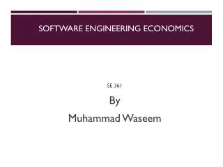
TPS II System Architecture- variant on COCOMO II book architecture … … … … … … … • Companies • Travel agents • About 10/region Clients … … … Local Concentrators Server … Regional Concentrators 1 N Financial DB DB Server Services DB
TPS II Concept of Operation • Clients prepare and send travel-itinerary requests to local concentrator • Package of air, rail, car, hotel reservation requests • Local concentrators validate requests and forward them to regional concentrators at server • Usually about 10 local concentrators per region • N Regional concentrators use DB server to develop best-match travel itinerary package • Send back to clients via local concentrators • Multiprocessor overhead due to resource contention, coordination
COTS vs. New Development Cost Tradeoff: TPS II • Build special version of server systems functions • To reduce COTS server software overhead, improve transaction throughput • Server systems software size: 20,700 SLOC • Server systems, library integration, status monitoring • COTS license tradeoffs vs. number of regional concentrators N • Need 10 N licenses for local concentrators • $1K each for acquisition, $1K each for 5-year maintenance
COTS/New Development Cost Tradeoff Analysis COTS $K New Development $K • Software • Cost to acquire 100 606 • Integrate & test 100 Included • Run-time licenses 10N Not applicable • 5-year maintenance 10N151 200 + 20N 757 • Server 250 + 20N250+20N • Total 450 + 40N 1007 + 20N
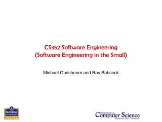
COTS/New Development Cost Tradeoff COTS 1200 1000 Life Cycle Cost, $K 800 New 600 400 200 10 20 30 40 50 Number of Regional Concentrators, N • Now, we need to address the benefit tradeoffs
TPS Decision 1How Many Regional Concentrators in Server? Performance Parameters N, number of processors N = ? S, processor speed (MOPS/sec) S = 1000 P, processor overhead (MOPS/sec) P = 200 M, multiprocessor overhead factor M = 80 [overhead=M(N-1) MOPS/sec] T, transaction processing time (MOPS/TR) T = 1.0 Performance (TR/sec) MOPS/sec available for processing MOPS/TR required per transaction N[S-P-M(N-1)] T E(N) = E(N) =
TPS Performance, E(N) E(N) = KOPS/sec available for processing KOPS/sec required per transaction N [ 1000-200-80(N-1)] 1.0 = N [1000-200+80)-80N2 = 880N – 80N2 = 80N(11-N) dE(N) dN 160N* = 880 N* = 5.5 E(N)* = 2440 = 0 = = 880 - 160N*
TPS throughout: E(N) versus number of processors, N E(N) (tr/sec) Number of processors N
TPS Decision 2Which Operating System? E(N) = N(1000-200-50(N-1)) Option B: E(N) = = 840N-40N2 1.0 = 40N(21-N) For N = 10, E(N) = 40(10)(11) = 4400
Cost-Effectiveness Comparison: TPS II Options A, B Option B E(N) = 40N(21 – N) C(N) = 1007 + 20N 5000 4000 3000 2000 1000 0 450 650 1207 0 500 1000 1500 Cost C, $K
Segments of Production Function Output Input High payoff Diminishing returns Investment
X Production Function Achievable output = F (input consumed) -Assuming only technologically efficient pairs: • No higher level of output achievable, using given input Output Input PF is nonnegative PF is nondecreasing
Natural speech input Tertairy application functions Animated displays Secondary application functions User amenities Value of software product to organization Main application functions Basic application functions Operating System Data management system Investment High-payoff Diminishing returns Cost of software product
Frequently Gold-Plating Instant response Pinpoint accuracy Unbalanced systems Usually Not Gold-Plating Humanized input Humanized output Sometimes Gold-Plating Highly generalized control, data structures Sophisticated command languages General-purpose utilities Automatic trend analysis Agents with attitudes Animated displays “everything for everybody” Modularity, info. hiding Measurement, diagnostics Software Gold-Plating
P11 P12 P13 P21 P22 P23 Modular Transaction Processing System Module 1 E(2 x 3) = 2 x E(3) = 3840 vs. 2400 1 Trans. in Processed Transaction out 2 Module 2
Software Project Diseconomies of Scale SLOC Output 1 + x PM = C (KSLOC) Person – Months Input • The best way to combat diseconomies of scale is to Reduce the Scale
Cost-Effectiveness Decision Criteria • Maximum available budget • Minimum performance requirement • Maximum effectiveness/cost ratio • Maximum effectiveness – cost difference • Return on investment (ROI) • Composite alternatives
B 4400 E (tr/sec) P Q A 2400 Z Y X 1207 450 650 1007 Production Functions for TPS II Options A, B
2400 R 2000 L Eff/Cost = 8 1600 E (tr/sec) 1200 K Eff/Cost = 3.69 800 400 100 200 300 400 500 600 700 C, $K Maximum Effectiveness/Cost Ratio
5000 4400 B-Build new OS 4000 3000 3193 2400 A-Accept available OS Throughput E(TR/sec) 2000 1750 1207 1000 650 0 500 1000 1500 Cost C, $K Maximum Effectiveness-Cost Difference
5 4 3 ROI = 2.67 E-C 2.60 C 2 A B 1 0 500 1000 1500 Cost C ($K) Return on Investment ROI
E 4400 E (r/sec) 2400 450 650 1007 1207 C, $K Production Function for TPS Composite Alternative
Summary – Cost-Effectiveness Analysis • Microeconomic concepts help structure, resolve software decision problems • Cost-effectiveness • Production functions • Economies of scale • C-E decision criteria • No single decision criterion dominates others • Each is best for some situations • Need to perform sensitivity analysis: • Slightly altered situation doesn’t yield bad decision