Predicting Selling Price with Multiple Regression

1. Chapter 13: Multiple Regression Section 13.1: How Can We Use Several Variables to Predict a Response?

2. Learning Objectives • Regression Models • The Number of Explanatory Variables • Plotting Relationships • Interpretation of Multiple Regression Coefficients • Summarizing the Effect While Controlling for a Variable • Slopes in Multiple Regression and in Bivariate Regression • Importance of Multiple Regression

3. Learning Objective 1:Regression Models • The model that contains only two variables, x and y, is called a bivariate model

4. Learning Objective 1:Regression Models • Suppose there are two predictors, denoted by x1 and x2 • This is called a multiple regression model

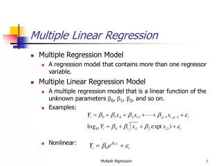
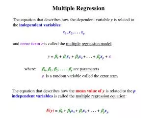
5. Learning Objective 1:Multiple Regression Model • The multiple regression model relates the mean µy of a quantitative response variable y to a set of explanatory variables x1, x2,…

6. Learning Objective 1:Multiple Regression Model • Example: For three explanatory variables, the multiple regression equation is:

7. Learning Objective 1:Multiple Regression Model • Example: The sample prediction equation with three explanatory variables is:

8. Learning Objective 1:Example: Predicting Selling Price Using House and Lot Size • The data set “house selling prices” contains observations on 100 home sales in Florida in November 2003 • A multiple regression analysis was done with selling price as the response variable and with house size and lot size as the explanatory variables

9. Learning Objective 1:Example: Predicting Selling Price Using House and Lot Size • Output from the analysis:

10. Learning Objective 1:Example: Predicting Selling Price Using House and Lot Size • Prediction Equation: where y = selling price, x1=house size and x2 = lot size

11. Learning Objective 1:Example: Predicting Selling Price Using House and Lot Size • One house listed in the data set had house size = 1240 square feet, lot size = 18,000 square feet and selling price = $145,000 • Find its predicted selling price:

12. Learning Objective 1:Example: Predicting Selling Price Using House and Lot Size • Find its residual: • The residual tells us that the actual selling price was $37,724 higher than predicted

13. Learning Objective 2:The Number of Explanatory Variables • You should not use many explanatory variables in a multiple regression model unless you have lots of data • A rough guideline is that the sample size n should be at least 10 times the number of explanatory variables

14. Learning Objective 3:Plotting Relationships • Always look at the data before doing a multiple regression • Most software has the option of constructing scatterplots on a single graph for each pair of variables • This is called a scatterplot matrix

15. Learning Objective 3:Plotting Relationships

16. Learning Objective 4:Interpretation of Multiple Regression Coefficients • The simplest way to interpret a multiple regression equation looks at it in two dimensions as a function of a single explanatory variable • We can look at it this way by fixing values for the other explanatory variable(s)

17. Learning Objective 4:Interpretation of Multiple Regression Coefficients Example using the housing data: • Suppose we fix x1 = house size at 2000 square feet • The prediction equation becomes:

18. Learning Objective 4:Interpretation of Multiple Regression Coefficients • Since the slope coefficient of x2 is 2.84, the predicted selling price increases by $2.84 for every square foot increase in lot size when the house size is 2000 square feet • For a 1000 square-foot increase in lot size, the predicted selling price increases by 1000(2.84) = $2840 when the house size is 2000 square feet

19. Learning Objective 4:Interpretation of Multiple Regression Coefficients Example using the housing data: • Suppose we fix x2 = lot size at 30,000 square feet • The prediction equation becomes:

20. Learning Objective 4:Interpretation of Multiple Regression Coefficients • Since the slope coefficient of x1 is 53.8, for houses with a lot size of 30,000 square feet, the predicted selling price increases by $53.80 for every square foot increase in house size

21. Learning Objective 4:Interpretation of Multiple Regression Coefficients • In summary, an increase of a square foot in house size has a larger impact on the selling price ($53.80) than an increase of a square foot in lot size ($2.84) • We can compare slopes for these explanatory variables because their units of measurement are the same (square feet) • Slopes cannot be compared when the units differ

22. Learning Objective 5:Summarizing the Effect While Controlling for a Variable • The multiple regression model assumes that the slope for a particular explanatory variable is identical for all fixed values of the other explanatory variables

23. Learning Objective 5:Summarizing the Effect While Controlling for a Variable • For example, the coefficient of x1 in the prediction equation: is 53.8 regardless of whether we plug in x2 = 10,000 or x2 = 30,000 or x2 = 50,000

24. Learning Objective 5:Summarizing the Effect While Controlling for a Variable

25. Learning Objective 6:Slopes in Multiple Regression and in Bivariate Regression • In multiple regression, a slope describes the effect of an explanatory variable while controlling effects of the other explanatory variables in the model

26. Learning Objective 6:Slopes in Multiple Regression and in Bivariate Regression • Bivariate regression has only a single explanatory variable • A slope in bivariate regression describes the effect of that variable while ignoring all other possible explanatory variables

27. Learning Objective 7:Importance of Multiple Regression • One of the main uses of multiple regression is to identify potential lurking variables and control for them by including them as explanatory variables in the model

28. Chapter 13:Multiple Regression Section 13.2 Extending the Correlation and R-Squared for Multiple Regression

29. Learning Objectives • Multiple Correlation • R-squared • Properties of R2

30. Learning Objective 1:Multiple Correlation • To summarize how well a multiple regression model predicts y, we analyze how well the observed y values correlate with the predicted values • The multiple correlation is the correlation between the observed y values and the predicted values • It is denoted by R

31. Learning Objective 1:Multiple Correlation • For each subject, the regression equation provides a predicted value • Each subject has an observed y-value and apredicted y-value

32. Learning Objective 1:Multiple Correlation • The correlation computed between all pairs of observed y-values and predicted y-values is the multiple correlation, R • The larger the multiple correlation, the better are the predictions of y by the set of explanatory variables

33. Learning Objective 1:Multiple Correlation • The R-value always falls between 0 and 1 • In this way, the multiple correlation ‘R’ differs from the bivariate correlation ‘r’ between y and a single variable x, which falls between -1 and +1

34. Learning Objective 2:R-squared • For predicting y, the square of R describes the relative improvement from using the prediction equation instead of using the sample mean,

35. Learning Objective 2:R-squared • The error in using the prediction equation to predict y is summarized by the residual sum of squares:

36. Learning Objective 2:R-squared • The error in using to predict y is summarized by the total sum of squares:

37. Learning Objective 2:R-squared • The proportional reduction in error is:

38. Learning Objective 2:R-squared • The better the predictions are using the regression equation, the larger R2 is • For multiple regression, R2 is the square of the multiple correlation, R

39. Learning Objective 2:Example: How Well Can We Predict House Selling Prices? • For the 100 observations on y = selling price, x1 = house size, and x2 = lot size, a table, called the ANOVA (analysis of variance) table was created • The table displays the sums of squares in the SS column

40. Learning Objective 2:Example: How Well Can We Predict House Selling Prices? • The R2value can be created from the sums of squares in the table

41. Learning Objective 2:Example: How Well Can We Predict House Selling Prices? • Using house size and lot size together to predict selling price reduces the prediction error by 71%, relative to using alone to predict selling price

42. Learning Objective 2:Example: How Well Can We Predict House Selling Prices? • Find and interpret the multiple correlation • There is a strong association between the observed and the predicted selling prices • House size and lot size are very helpful in predicting selling prices

43. Learning Objective 2:Example: How Well Can We Predict House Selling Prices? • If we used a bivariate regression model to predict selling price with house size as the predictor, the r2 value would be 0.58 • If we used a bivariate regression model to predict selling price with lot size as the predictor, the r2 value would be 0.51

44. Learning Objective 2:Example: How Well Can We Predict House Selling Prices? • The multiple regression model has R2 0.71, so it provides better predictions than either bivariate model

45. Learning Objective 2:Example: How Well Can We Predict House Selling Prices?

46. Learning Objective 2:Example: How Well Can We Predict House Selling Prices? • The single predictor in the data set that is most strongly associated with y is the house’s real estate tax assessment • (r2 = 0.679) • When we add house size as a second predictor, R2 goes up from 0.679 to 0.730 • As other predictors are added, R2 continues to go up, but not by much

47. Learning Objective 2:Example: How Well Can We Predict House Selling Prices? • R2 does not increase much after a few predictors are in the model • When there are many explanatory variables but the correlations among them are strong, once you have included a few of them in the model, R2 usually doesn’t increase muchmore when you add additional ones

48. Learning Objective 2:Example: How Well Can We Predict House Selling Prices? • This does not mean that the additional variables are uncorrelated with the response variable • It merely means that they don’t add much new power for predicting y, given the values of the predictors already in the model

49. Learning Objective 3:Properties of R2 • The previous example showed that R2 for the multiple regression model was larger than r2 for a bivariate model using only one of the explanatory variables • A key factor of R2 is that it cannot decrease when predictors are added to a model

50. Learning Objective 3:Properties of R2 • R2 falls between 0 and 1 • The larger the value, the better the explanatory variables collectively predict y • R2 =1 only when all residuals are 0, that is, when all regression predictions are prefect • R2 = 0 when the correlation between y and each explanatory variable equals 0