Efficient market Hypothesis
Efficient market Hypothesis. BKM: 8.1, 8.2. Apparent Patterns in Prices. Random Walk in Prices. Math review: ln (x)- ln (y)= ln (x/y) But then this implies that the stated rate with continuous compounding follows a constant+white noise process!

Efficient market Hypothesis
E N D
Presentation Transcript
Efficient market Hypothesis BKM: 8.1, 8.2
Random Walk in Prices • Math review: ln(x)-ln(y)=ln(x/y) • But then this implies that the stated rate with continuous compounding follows a constant+white noise process! To a reasonable approximation we can say that the effective excess return also follows a constant plus white noise process.
Efficient market Hypothesis • The finding that returns follow a “constant + white noise” process is the necessary consequence of intelligent investors competing to discover relevant information. • Efficient Market Hypothesis: • As soon as new information is revealed, prices immediatelyadjust to reflect that information so that E[re] for any stock equals the fair risk premium for that stock. • That is, excess returns follow a constant+white noise process.
Three Versions of the Efficient Market Hypothesis • Weak-Form EMH • Stock prices immediately reflect all information contained in the history of stock trading. • Semistrong-Form EMH • Stock prices immediately reflect all publicly-available information. • Strong-Form EMH • Stock prices immediately reflect all relevant information including inside information.
Three Versions of the Efficient Market Hypothesis • Past prices are a subset of public information • Public information is a subset of all information. • Hence: • What if markets are semistrong-form efficient. • What do we know about weak-form efficiency? • The market must also be weak-form efficient. • If prices reflect all public information, then they must reflect information in past prices. • What if markets are strong-form efficient. • What do we know about weak-form efficiency? • The market must also be weak-form efficient • If prices reflect all information, including insider information, then they must reflect public information.
Three Versions of the Efficient Market Hypothesis • Past prices are a subset of public information • Public information is a subset of all information. • Hence: • What if markets are not weak-form efficient? • What do we know about semistrong-form efficiency? • The market cannot be semistrong-form efficient. • If prices do not reflect information in past prices, then they can’t reflect all public information. • What if markets are not semistrong-form efficient? • What do we know about strong-form efficiency? • The market cannot be strong-form efficient. • If prices do not reflect all public information, then they can’t reflect all information.
Three Versions of the Efficient Market Hypothesis It is possible for the market to be weak form efficient, but not semi- or strong form efficient. It is possible for the market to be semi-strong form efficient, but not strong form efficient.
How efficient are markets? My view: Almost semi-strong form efficient
Abnormal Return • Review • The risk premium is the expected excess return. • We can estimate the risk premium using the historical average. • One test of market efficiency is to test if the historical average excess return is above or below the fair value (k) for the risk premium. • Probably won’t be exactly equal because of sampling error.
Abnormal Returns following Earnings Announcements Source: Patell and Wolfson (1984)
Mutual Fund Performance • Most actively-managed funds do not beat market indices. Source: Malkiel (2003)
Mutual Fund Performance • There is not much persistence in mutual fund performance. • How well did the top 20 Equity Funds in the 1980s perform in the 1990s?
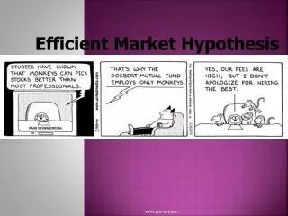
Assume Semi-Strong Form • Do analysts still add value? • Maybe just hire a blind monkey to throw darts on the Wall Street Journal to select stocks.
Efficient Markets • In an “efficient” market, there will be rewards to doing research. Research Conducted Rewards for Research Market Efficiency
Efficient Markets • Who is getting these rewards? • Open research question . . . • Rewards will be highest for those managing large portfolios. • Example: • Suppose you have $10,000 invested • Suppose research will yield a guaranteed increase in return of 0.1% over the next year • You get $10 woo-hoo! • Now suppose you have $10 billion invested . . . .
Forecast Accuracy • Measure expected deviation of forecast from outcome. • E(outcome-forecast) • Interpretation: crank out an infinite number of observations from the PDF, subtract your forecast from each outcome, and find the average of this difference across all outcomes. • E(x-E[x]) is always zero. • The expectation is accurate and unbiased. • We don’t ever know the true PDF, so we can’t ever calculate the true risk premium. • However, we can estimate it as a simple average of past excess returns because the risk premium does not change over time.
Measuring Uncertainty • For some stocks we can be more confident about our forecast than others.
Variation in excess returns • Excess return: • Virtually all of the variation in excess returns comes from variation in the stock return. • For practical purposes we often consider the return on short-term t-bills to be constant. • How can we measure variation in returns?
Discrete Examples • Investment #1 • E[r]=3.75% • Investment #2 • E[r]=3.75%
Variance • When using E[r] as a forecast, we know the bias will always be zero • E[r-E[r]] • Investment #1: • E[r-E[r]]=.75*(.10-.0375)+.25*(-.15-.0375)=0 • Investment #2: • E[r-E[r]]=1*(.0375-.0375) =0 • Not a very helpful measure of variation.
Variance • How about finding the expected squared bias? • Investment #1 • E[(r-E[r])2]=.75*(.10-.0375)2+.25*(-.15-.0375)2=0.0117 • Investment #2 • E[(r-E[r])2]=1*(.0375-.0375) 2=0 • The expected squared bias, or the expected squared deviation from the mean is the variance.
Variance • For a discrete PDF with n outcomes the true variance is: • We never know the true PDF for stock returns • But we do observe outcomes for stock returns • Estimate the variance as the average squared deviation from mean.
Estimation • Example: • Sample of returns: 0.10, 0.05, 0, -.03 • Step 1: • Step 2:
Standard Deviation • Standard Deviation = Square Root(variance) • Both for discrete and continuous PDF’s • Notation • Variance: s2 • Standard Deviation: s
Examples Stdev=0.018 Stdev=0.034
Standard Deviation • What does standard deviation tell us that variance doesn’t? • Discrete Random Variable • Not much • Continuous normal PDF • Helps us directly answer the following questions: • How likely do I get wiped out? • Is there some chance I smack a home run? • What outcomes are most likely to happen?

