Dividing Polynomials
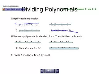
Dividing Polynomials. divisor. Dividing by a Monomial . If the divisor only has one term, split the polynomial up into a fraction for each term. Now reduce each fraction. 3 x 3. 4 x 2. x. 2. 1. 1. 1. 1. Long Division of Polynomials.


Dividing Polynomials
E N D
Presentation Transcript
divisor Dividing by a Monomial If the divisor only has one term, split the polynomial up into a fraction for each term. Now reduce each fraction. 3x3 4x2 x 2 1 1 1 1
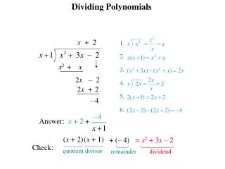
Long Division of Polynomials Now multiply by the divisor and put the answer below. Bring down the next number or term 32 698 First divide 3 into 6 or x into x2 Now divide 3 into 5 or x into 11x So we found the answer to the problem x2 + 8x – 5 x – 3 or the problem written another way: If the divisor has more than one term, perform long division. You do the same steps with polynomial division as with integers. Let's do two problems, one with integers you know how to do and one with polynomials and copy the steps. Subtract (which changes the sign of each term in the polynomial) x + 11 2 1 Multiply and put below x - 3 x2 + 8x - 5 Remainder added here over divisor 64 x2 – 3x subtract 5 8 11x - 5 32 11x - 33 This is the remainder 26 28
Write out with long division including 0y for missing term Divide y into y2 Divide y into -2y Let's Try Another One If any powers of terms are missing you should write them in with zeros in front to keep all of your columns straight. Subtract (which changes the sign of each term in the polynomial) y - 2 Multiply and put below Bring down the next term Multiply and put below y + 2 y2 + 0y + 8 Remainder added here over divisor y2 + 2y subtract -2y + 8 - 2y - 4 This is the remainder 12
REMAINDER THEOREM Let f be a polynomial function. If f (x) is divided by x – c, then the remainder is f (c). Let’s look at an example to see how this theorem is useful. So the remainder we get in synthetic division is the same as the answer we’d get if we put -2 in the function. The root of x + 2 = 0 is x = -2 using synthetic division let’s divide by x + 2 -2 2 -3 2 -1 -4 14 -32 2 -7 16 -33 the remainder Find f(-2)
FACTOR THEOREM Let f be a polynomial function. Then x – c is a factor of f (x) if and only if f (c) = 0 -3 -4 5 0 8 12 -51 153 -4 17 -51 161 If and only if means this will be true either way: 1. If f(c) = 0, then x - c is a factor of f(x) 2. If x - c is a factor of f(x) then f(c) = 0. Try synthetic division and see if the remainder is 0 Opposite sign goes here NO it’s not a factor. In fact, f(-3) = 161 We could have computed f(-3) at first to determine this. Not = 0 so not a factor
Set divisor = 0 and solve. Put answer here. x + 3 = 0 so x = - 3 Bring first number down below line Multiply these and put answer above line in next column Multiply these and put answer above line in next column Multiply these and put answer above line in next column Synthetic Division There is a shortcut for long division as long as the divisor is x – k where k is some number. (Can't have any powers on x). 1 - 3 1 6 8 -2 - 3 Add these up - 9 3 Add these up Add these up 1 x2 + x 3 - 1 1 This is the remainder Put variables back in (one x was divided out in process so first number is one less power than original problem). So the answer is: List all coefficients (numbers in front of x's) and the constant along the top. If a term is missing, put in a 0.
Set divisor = 0 and solve. Put answer here. x - 4 = 0 so x = 4 Bring first number down below line Multiply these and put answer above line in next column Multiply these and put answer above line in next column Multiply these and put answer above line in next column Multiply these and put answer above line in next column Let's try another Synthetic Division 0 x3 0 x 1 4 1 0 - 4 0 6 4 Add these up 16 48 192 Add these up Add these up Add these up 1 x3 + x2 + x + 4 12 48 198 This is the remainder Now put variables back in (remember one x was divided out in process so first number is one less power than original problem so x3). So the answer is: List all coefficients (numbers in front of x's) and the constant along the top. Don't forget the 0's for missing terms.
Bring first number down below line Multiply these and put answer above line in next column Multiply these and put answer above line in next column Multiply these and put answer above line in next column Let's try a problem where we factor the polynomial completely given one of its factors. You want to divide the factor into the polynomial so set divisor = 0 and solve for first number. - 2 4 8 -25 -50 - 8 Add these up 0 50 Add these up Add these up No remainder so x + 2 IS a factor because it divided in evenly 4 x2 + x 0 - 25 0 Put variables back in (one x was divided out in process so first number is one less power than original problem). So the answer is the divisor times the quotient: List all coefficients (numbers in front of x's) and the constant along the top. If a term is missing, put in a 0. The second factor is the difference of squares so factor it.
Our goal in this section is to learn how we can factor higher degree polynomials. For example we want to factor: We could randomly try some factors and use synthetic division and know by the factor theorem that if the remainder is 0 then we have a factor. We might be trying things all day and not hit a factor so in this section we’ll learn some techniques to help us narrow down the things to try. The first of these is called Descartes Rule of Signs named after a French mathematician that worked in the 1600’s. Rene Descartes 1596 - 1650
Descartes’ Rule of Signs Let f denote a polynomial function written in standard form. The number of positive real zeros of f either equals the number of sign changes of f (x) or else equals that number less an even integer. The number of negative real zeros of f either equals the number of sign changes of f (-x) or else equals that number less an even integer. 1 2 starts Pos. changes Neg.changes Pos. There are 2 sign changes so this means there could be 2 or 0 positive real zeros to the polynomial.
Use Descartes’ Rule of Signs to determine how many positive and how many negative real zeros the polynomial may have. Counting multiplicities and complex (imaginary) zeros, the total number of zeros will be the same as the degree of the polynomial. 1 starts Neg. changes Pos. There is one sign change so there is one positive real zero. starts Pos. Never changes There are no negative real zeros. Descartes rule says one positive and no negative real zeros so there must be 4 complex zeros for a total of 5. We’ll learn more complex zeros in Section 4.7.
Back to our original polynomial we want to factor: 1 We’d need to try a lot of positive or negative numbers until we found one that had 0 remainder. To help we have: The Rational Zeros Theorem What this tells us is that we can get a list of the POSSIBLE rational zeros that might work by taking factors of the constant divided by factors of the leading coefficient. Both positives and negatives would work for factors 1, 2 Factors of the constant 1 Factors of the leading coefficient
1 1 1 -3 -1 2 1 2 -1 -2 1 2 -1 -2 0 So a list of possible things to try would be any number from the top divided by any from the bottom with a + or - on it. In this case that just leaves us with 1 or 2 1, 2 1 Let’s try 1 YES! It is a zero since the remainder is 0 We found a positive real zero so Descartes Rule tells us there is another one Since 1 is a zero, we can write the factor x - 1, and use the quotient to write the polynomial factored.
1 1 2 -1 -2 1 3 2 1 3 2 0 We could try 2, the other positive possible. IMPORTANT: Just because 1 worked doesn’t mean it won’t work again since it could have a multiplicity. 1, 2 1 Let’s try 1 again, but we try it on the factored version for the remaining factor (once you have it partly factored use that to keep going---don't start over with the original). YES! the remainder is 0 Once you can get it down to 3 numbers here, you can put the variables back in and factor or use the quadratic formula, we are done with trial and error.
Let’s take our polynomial then and write all of the factors we found: There ended up being two positive real zeros, 1 and 1 and two negative real zeros, -2, and -1. In this factored form we can find intercepts and left and right hand behavior and graph the polynomial Plot intercepts Left & right hand behavior Touches at 1 crosses at -1 and -2. “Rough” graph
Let’s try another one from start to finish using the theorems and rules to help us. Using the rational zeros theorem let's find factors of the constant over factors of the leading coefficient to know what numbers to try. 1, 3, 9 factors of constant 1, 2 factors of leading coefficient So possible rational zeros are all possible combinations of numbers on top with numbers on bottom:
1 2 3 4 starts Pos. changes Neg. changes Pos. Changes Neg. Changes Pos. starts Pos. Stays positive Let’s see if Descartes Rule helps us narrow down the choices. No sign changes in f(x) so no positive real zeros---we just ruled out half the choices to try so that helps! 4 sign changes so 4 or 2 or 0 negative real zeros.
-1 2 13 29 27 9 -1 2 11 18 9 -2 -11 -18 -9 -2 - 9 -9 2 11 18 9 0 2 9 9 0 Let’s try -1 Yes! We found a zero. Let’s work with reduced polynomial then. Yes! We found a zero. Let’s work with reduced polynomial then. Let’s try -1 again Yes! We found another one. We are done with trial and error since we can put variables back in and solve the remaining quadratic equation. So remaining zeros found by setting these factors = 0 are -3/2 and -3. Notice these were in our list of choices.
Let’s solve the equation: To do that let’s consider the function If we find the zeros of the function, we would be solving the equation above since we want to know where the function = 0 By Descartes Rule: There is one sign change in f(x) so there is one positive real zero. There are 2 sign changes in f(-x) so there are 2 or 0 negative real zeros. Using the rational zeros theorem, the possible rational zeros are: 1, 5 1, 2
1 2 -3 -3 -5 5 2 -3 -3 -5 2 -1 -4 10 35 160 2 -1 -4 -9 2 7 32 155 1 is not a zero and f(1) = -9 Let’s try 1 5 is not a zero and f(5) = 155 Let’s try 5 On the next screen we’ll plot these points and the y intercept on the graph and think about what we can tell about this graph and its zeros.
155 is a lot higher than this but that gives us an idea it’s up high f(5) = 155 To join these points in a smooth, continuous curve, you would have to cross the x axis somewhere between 1 and 5. This is the Intermediate Value Theorem in action. We can see that since Descartes Rule told us there was 1 positive real zero, that is must be between 1 and 5 so you wouldn’t try 1/2, but you'd try 5/2 instead. f(0) = -5 f(1) = -9
Intermediate Value TheoremLet f denote a polynomial function. If a < b and if f(a) and f(b) are of opposite sign, then there is at least one zero of f between a and b. f(5) = 155 In our illustration, a = 1 and b =5 So if we find function values for 2 different x’s and one is positive and the other negative, there must be a zero of the function between these two x values In our illustration, f(a) = -9 and f(b) = 155 which are opposite signs f(1) = -9
-1 1 8 -1 0 2 -1 -7 8 -8 1 7 -8 8 -6 We use this theorem to approximate zeros when they are irrational numbers. The function below has a zero between -1 and 0. We’ll use the Intermediate Value Theorem to approximate the zero to one decimal place. First let’s verify that there is a zero between -1 and 0. If we find f(-1) and f(0) and they are of opposite signs, we’ll know there is a zero between them by the Intermediate Value Theorem. So f(-1) = -6 and f(0) = 2These are opposite signs.
neg Does the sign change occur between f(-1) and f(-0.5) or between f(-0.5) and f(0)? pos -1 -0.5 1 8 -1 0 2 -0.5 -3.75 2.375 -1.1875 1 7.5 -4.75 2.375 0.8125 pos f(-1) = -6 The graph must cross the x-axis somewhere between -1 and 0 f(-0.7) = -0.9939 Let’s try half way between at x = - 0.5 Sign change f(-0.6) = 0.0416 f(-0.5) = 0.8125 So let’s try something between -1 and - 0.5. Let’s try - 0.7. Do this with synthetic division or direct substitution. - 0.6 is the closest to zero so this is the zero approximated to one decimal place f(0) = 2 Notice that the sign change is between - 0.7 and - 0.6