Download
1 / 58
640 likes | 1.5k Vues
PowerWorld Simulator OPF and Locational Marginal Prices. Presentation Goals. Provide background on Optimal Power Flow (OPF) Problem Show how OPF is implemented in PowerWorld Simulator OPF Demonstrate how Simulator OPF can be used to solve small and large problems

E N D
Presentation Goals • Provide background on Optimal Power Flow (OPF) Problem • Show how OPF is implemented in PowerWorld Simulator OPF • Demonstrate how Simulator OPF can be used to solve small and large problems • Provide hands-on Simulator OPF examples
Optimal Power Flow Overview • The goal of an optimal power flow (OPF) is to determine the “best” way to instantaneously operate a power system. • Usually “best” = minimizing operating cost. • OPF considers the impact of the transmission system • We’ll introduce OPF initially ignoring the transmission system
“Ideal” Power Market - No Transmission System Constraints • Ideal power market is analogous to a lake. Generators supply energy to lake and loads remove energy. • Ideal power market has no transmission constraints • Single marginal cost associated with enforcing constraint that supply = demand • buy from the least cost unit that is not at a limit • this price is the marginal cost
Market Marginal Cost is Determined from Net Gen Costs Below are some graphs associated with this two bus system. The graph on left shows the marginal cost for each of the generators. The graph on the right shows the system supply curve, assuming the system is optimally dispatched. Current generator operating point
80.0 60.0 40.0 Marginal Cost ($ / MWh) 20.0 0.0 60 100 140 180 Total Generation (GW) Variation in Marginal Cost for Northeast U.S. For each value of generation there is a single, system-wide marginal cost
Real Power Market • Different operating regions impose constraints -- total demand in region must equal total supply • Transmission system imposes constraints on the market • Marginal costs become localized • Requires solution by an optimal power flow
Optimal Power Flow (OPF) • Minimize cost function, such as operating cost, taking into account realistic equality and inequality constraints • Equality constraints • bus real and reactive power balance • generator voltage setpoints • area MW interchange • transmission line/transformer/interface flow limits
Optimal Power Flow (OPF) • Inequality constraints • transmission line/transformer/interface flow limits • generator MW limits • generator reactive power capability curves • bus voltage magnitudes (not yet implemented in Simulator OPF) • Available Controls • generator MW outputs • Load MW demands • phase shifters
OPF Solution Methods • Non-linear approach using Newton’s method • handles marginal losses well, but is relatively slow and has problems determining binding constraints • Linear Programming • fast and efficient in determining binding constraints, but has difficulty with marginal losses.
LP OPF • Two approaches are possible • primal • take a feasible solution and make it optimal • dual • take an optimal solution and make it feasible • PowerWorld Simulator OPF only includes a primal approach (currently)
Primal LP OPF Solution Algorithm • Solution iterates between • solving a full ac power flow solution • enforces real/reactive power balance at each bus • enforces generator reactive limits • system controls are assumed fixed • takes into account non-linearities • solving a primal LP • changes system controls to enforce linearized constraints while minimizing cost
LP Solution • Problem is setup to be initially feasible through the use of slack variables • slack variables have high marginal costs; LP algorithm will remove them if at all possible • Slack variables are used to enforce • area/super area MW constraints • MVA line/transformer constraints • MW interface constraints
Two Bus Example - No Constraints With no overloads the OPF matches the economic dispatch Transmission line is not overloaded Marginal cost of supplying power to each bus (locational marginal costs)
Two Bus Example with Constrained Line With the line loaded to its limit, additional load at Bus A must be supplied locally, causing the marginal costs to diverge.
Three Bus (B3) Example • Consider a three bus case (bus 1 is system slack), with all buses connected through 0.1 pu reactance lines, each with a 100 MVA limit • Let the generator marginal costs be • Bus 1: 10 $ / MWhr; Range = 0 to 400 MW • Bus 2: 12 $ / MWhr; Range = 0 to 400 MW • Bus 3: 20 $ / MWhr; Range = 0 to 400 MW • Assume a single 180 MW load at bus 2
Solving the LP OPF • All LP OPF commands are accessed from the LP OPF menu item. • Before solving, we first need to specify what constraints to enforce • Select LP OPF, OPF Area Records to turn on area constraint; set AGC Status to “OPF” • Initially we’ll disable line MVA enforcement; Select LP OPF, Options; check “Disable Line/Transformer MVA Line Limit Enforcement”
B3 with Line Limits NOT Enforced Line from Bus 1 to Bus 3 is over- loaded; all buses have same marginal cost
Line Limit Enforcement • Previous LP tableau wasPG1 PG2 PG3 S1 b1.00 1.00 1.00 1.00 0.00 • Line limit tableau isPG1 PG2 PG3 S1 S2 b1.00 1.0 1.00 1.00 0.00 0.000.00 -0.33 -0.66 0.00 1.00 -0.20 • Second row is from enforcing the line flow MVA constraint
B3 with Line Limits Enforced LP OPF redispatches to remove violation. Bus marginal costs are now different.
Verify Bus 3 Marginal Cost One additional MW of load at bus 3 raised total cost by 14 $/hr, as G2 went up by 2 MW and G1 went down by 1MW
Why is bus 3 LMP = $14 /MWh • All lines have equal impedance. Power flow in a simple network distributes inversely to impedance of path. • For bus 1 to supply 1 MW to bus 3, 2/3 MW would take direct path from 1 to 3, while 1/3 MW would “loop around” from 1 to 2 to 3. • Likewise, for bus 2 to supply 1 MW to bus 3, 2/3MW would go from 2 to 3, while 1/3 MW would go from 2 to 1to 3.
Why is bus 3 LMP = $ 14 / MWh? • With the line from 1 to 3 limited, no additional power flows are allowed on it. • To supply 1 more MW to bus 3 we need Pg1 + Pg2 = 1 MW 2/3 Pg1 + 1/3 Pg2 = 0; (no more flow on 1-3) • Solving requires we up Pg2 by 2 MW and drop Pg1 by 1 MW -- a net increase of $14.
Both lines into Bus 3 Congested For bus 3 loads above 200 MW, the load must be supplied locally. Then what if the bus 3 generator opens?
Case with G3 OpenedUnenforceable Constraints Both constraints can not be enforced. One is unenforce- able. Bus 3 marginal cost is arbitrary
Unenforceable Constraint Costs • If a constraint can not be enforced due to insufficient controls, the slack variable associated with enforcing that constraint can not be removed from the LP basis • marginal cost depends upon the assumed cost of the slack variable • this value is specified in the Maximum Violation Cost field on the LP OPF, Options dialog.
LP OPF, Options Dialog Disables enforcement of line constraints Enforcement tolerance deadband; needed because of system non- linearities Previously binding line constraints with loadings above this value remain in tableau Cost of unenforceable line violations Similar fields for interfaces
OPF Line/Transformer MVA Constraints Display Indicates if line is unenforceable Set to specify enforcement of individual lines Line loadings Marginal costs are non-zero only for lines that are active constraints
OPF Area Records Display Interpreting this value is difficult in areas with congestion Phase shifter control status AGC (automatic generation control) status must be set to “OPF” to include this are in the OPF objective function Set to indicate if branch and/or interface constraints in an area should be enforced
OPF Generator Records Display The OPF Generator Records display is similar to the Generator Records display, except it contains several LP OPF specific fields Current MW marginal cost Amount of change in MW during last OPF solution OPF MW Control specifies whether a particular generator is available for control
Hands-on: Three Bus Case • Load B3LP case. Select LP OPF, Primal LP to solve the case. Initially line limits are not enforced. • Select LP OPF, Options to view the options dialog • on the Constraint Options page enable the enforcement of line constraints • Use Solve LP OPF button on bottom of dialog to solve the case
Hands-on: Three Bus Case • View results using the LP OPF, OPF Areas, OPF Buses, OPF Gens and OPF Line/Transformer displays • on the OPF Line/Transformer display, toggle the Enforce MVA field to enable/disable the enforcement of individual lines. • verify that the marginal cost of enforcing the line overload is $ 6 / MVA/hr by changing the line limit and resolving. Why is it $6?
Hands-on: Three Bus Case • Increase the bus 3 load to 220 MW. Resolve with line enforcement active. What are the new LMPs? Why? • Open the generator at bus 3 and then resolve. Does this case have a solution? Why? Are the LMPs valid?
Modeling Generator Costs • Generator costs are modeled with either a cubic cost or piecewise linear cost function Cost model is specified on the generator dialog The LP OPF requires a piecewise linear model. Therefore any existing cubic models are automatically converted to piecewise linear before the solution, and then converted back afterward.
Automatic Conversion of Generator Cubic Cost Curves Conversion is determined based upon values shown on the LP OPF Dialog, General Options Page. Convert to either a specified number of points per curve or a specified MW per segment If unchecked then existing piecewise linear curves are overwritten
Comparison of Cubic and Piecewise Linear Marginal Cost Curves $ / MWh Continuous generator marginal cost curve Piecewise linear generator marginal cost curve with five segments This conversion may affect the final cost. Using more segments better approximates the original curve, but may take longer to solve
Super Areas • Super areas are a record structure used to hold a set of areas • Using super areas a number of areas can be dispatched as though they were a single area • For a super area to be used in the OPF, its AGC Status field must be “OPF”
Seven Bus Example - Dispatched as Three Separate Areas Contour of Bus LMPs Average LMP = $ 15.53 / MWh
Seven Bus Case Dispatched as One Super Area Contour of Bus LMPs Average LMP = $ 16.57 / MWh Net result: Lower cost, yet with higher LMPs
Hands-on: Seven bus case • Load the B7FlatLP case. Try to duplicate the results from the previous two slides. • What are the marginal costs of enforcing the line constraints? How do the system costs change if the line constraints are relaxed (i.e, not enforced)? For example, try solving without enforcing line 1 to 2.
Hands-on: Seven Bus Case • Modify the cost model for the generator at bus one. • How does changing from piece-wise linear to cubic affect the final solution? • How do the generation conversion parameters on the option dialog affect the results? • Try resolving the case with different lines removed from service.
LP Application: Profit Maximization on 30 Bus System The next slides illustrate how the OPF can be used to study the impact of bids on profit. Assume bus 13 generator has a true marginal cost of $ 7 / MWh.
Profit Maximization • If the bus 13 generator were paid its bus LMP * its output, its profit would beProfit = LMP * MW - 7 * MW • The question then is what should they bid to maximize their profit? This problem can be solved using the OPF with different assumed generator costs.
Profit Maximization Generator 13’s best response is to bid about $ 9.5 / MWh
Profit Maximization LMP contours with generator 13 maximizing its profit
Application of LP OPF to a Large System • Next case is based upon the FERC Form 715 1997 Summer Peak case filed by NEPOOL • case has 9270 buses and 2506 generators, representing a significant portion of the Eastern Interconnect transmission and generation • estimated cost data for most generators in NEPOOL, NYPP, PJM, ECAR • these regions were modeled as a super area • results developed by joint project between PowerWorld and U.S. Energy Information Administration
NEPOOL/NYPP/PJM/ECAR Supply Curve Super area has total generation of about 160 GW, with imports of 2620 MW Flat portion of curve at 10 $/MWhr repre- sents generators with default data
NYPP/NEPOOL Lower Voltage Transmission - Optimal Solution The constrained lines are shown with the large red pie charts