Introduction to Model Predictive Control Technology
Introduction to Model Predictive Control Technology. Hao-Yeh Lee P rocess S ystem E ngineering Laboratory Department of Chemical Engineering National Taiwan University. Outline. Introduction Model Forms for MPC Dynamic Matrix Control (DMC) SISO formulation MIMO formulation

Introduction to Model Predictive Control Technology
E N D
Presentation Transcript
Introduction to Model Predictive Control Technology Hao-Yeh Lee Process System Engineering Laboratory Department of Chemical Engineering National Taiwan University
Outline • Introduction • Model Forms for MPC • Dynamic Matrix Control (DMC) • SISO formulation • MIMO formulation • Quadratic Dynamic Matrix Control (QDMC) • MATLAB tools for MPC • Case Study • Conclusion
Introduction • The main idea of model predictive control (MPC) is to choose the control action by repeatedly solving on line an optimal control problem. • This aims at minimizing a performance criterion over a future horizon, possibly subject to constraints on the manipulated inputs and outputs, where the future behavior is computed according to a model of the plant.
Advantages of MPC • Easy to use for MIMO system and easy to handle process interactions • Easy to handle time delays, inverse response, as well as other difficult process dynamics. • Only few tuning parameters are needed.
A History of MPC • MAC, IDCOM (Richalet et al. , 1976, 1978) • using a discrete-time Finite Impulse Response (FIR) model. • Dynamic Matrix Control (DMC), (Cutler and Ramaker, 1979) • linear step response model for the plant • quadratic performance objective over a finite prediction horizon • future plant output behavior specified by trying to follow the setpoint as closely as possible • optimal inputs computed as the solution to a least-squares problem
A History of MPC (cont’d) • Quadratic Dynamic Matrix Control (QDMC), (García and Morshedi, 1984) • linear step response model for the plant • quadratic performance objective over a finite prediction horizon • future plant output behavior specified by trying to follow the setpoint as closely as possible subject to process constraints • optimal inputs computed as the solution to a quadratic program • Generalized Predictive Control (GPC) (Clarke et al., 1987) • Transfer function model for the plant • Nonlinear Model Predictive Control (NMPC)
Basic Elements of MPC • Reference Trajectory Specification • Process Output Prediction • Control Action Sequence Computation • Error Prediction Update
Model Forms for MPC • Convolution model • Step response model • Impulse response model • Discrete state-space model • Discrete transfer function model finite step response (FSR) finite impulse response (FIR)
Dynamic Matrix Control • Unconstrained Model Predictive Control
Step Response Model • For SISO system
Finite Step Response Model • :process output at time k • :step response coefficient at time i • :controller output at time k • :model horizon Define:
Finite Step Response Model (cont’d) • If the Hm is large enough, the process output will be approached to steady state for the stable process • The finite step response model (FSR) →
Impulse response model • It is easy to convert the impulse response model as step response model
The Concept of Moving Horizon Define: ∴
After Hcsteps, the manipulating variable rates are all the same, then
Process Output Prediction • Define the past input effect term: Dynamic matrix
Process Output Prediction (cont’d) • Define error prediction update term Define: Future input effect past input effect Future output
Control Action Sequence Computation • DMC control law
Control Action Sequence Computation(cont’d) • To apply the concept of moving horizon
MIMO system formulation • For nu × ny MIMO system • Step response model
Selection of Tuning Parameters • Systematic parameters • Sampling interval (Ts) • Ts should be small enough to capture the dynamics of the process, large enough to permit the on-line computations necessary for implementation • Model horizon (Hm) • Major tuning parameters • Prediction horizon (Hp) • Longer Hp tends to produce more aggressive control action, more overshoot, faster response and moresensitive to disturbances • Control horizon (Hc) • Control horizon should be less or equal to prediction horizon • The effect of increasing is very similar to prediction horizon
Selection of Tuning Parameters(cont’d) • Weighting parameters • Penalty factor ( f ) • A input weighting factor usually is set less than 10% of the output penalty to achieve good closed-loop performance. • Weighting matrix (G) • Output penalty matrix
Quadratic Dynamic Matrix Control • QDMC is the DMC extended to concern the system constraints • It uses quadratic programming technique to solve the optimization problem. • Quadratic programming form:
Process constraints • Manipulated variable constraints
Process constraints (cont’d) • Manipulated variable rate constraints
Process constraints (cont’d) • Output variable constraints
Quadratic Programming Control law:
Limitations of Existing Technology • impulse and step response models are limit application of the algorithm to strictly stable processes • sub-optimal solution of the dynamic optimization • constant output disturbance assumption • tuning is required to achieve nominal stability • model uncertainty is not addressed adequately
MATLAB Tools for MPC • MATLAB code for DMC • [yp,u,ym] = mpcsim(plant,model,Kmpc,tend,r,usat,... tfilter,dplant,dmodel,dstep) • Kmpc = mpccon(model,ywt,uwt,M,P) • plant = tfd2step(tfinal,delt2,nout,g1,...,g25) • plant = ss2step(phi, gam, c, d, tfinal) • MATLAB code for QDMC • [yp,u,ym] = cmpc(plant,model,ywt,uwt,M,P,tend,... r,ulim,ylim,tfilter,dplant,dmodel,dstep)
Case Study • 2x2 Example • Wood and Berry process
MATLAB Code for MPC • Setpoint change g11=poly2tfd(12.8,[16.7 1],0,1); g21=poly2tfd(6.6,[10.9 1],0,7); g12=poly2tfd(-18.9,[21.0 1],0,3); g22=poly2tfd(-19.4,[14.4 1],0,3); delt=3; ny=2; tfinal=90; model=tfd2step(tfinal,delt,ny,g11,g21,g12,g22); plant=model; P=6; M=2; ywt=[ ]; uwt=[1 1]; tend=30; r=[0 1]; ulim=[-inf -0.15 inf inf 0.1 100]; ylim=[ ]; [y,u]=cmpc(plant,model,ywt,uwt,M,P,tend,r,ulim,ylim); plotall(y,u,delt)
Disturbance rejection gd11=poly2tfd(3.8,[14.9 1],0,8.1); gd21=poly2tfd(4.9,[13.2 1],0,3.4); dmodel=tfd2step(tfinal,delt,ny,gd11,gd21); dplant=dmodel; r=[0 0]; dstep=1; tfilter = []; [y,u]=cmpc(plant,model,ywt,uwt,M,P,tend,r,ulim,ylim, tfilter,dplant,dmodel,dstep); plotall(y,u,delt)
Conclusion • The major advantage of the MPC algorithm is easy to handle multivariable system. • Quadratic dynamic matrix control can concern the system constraints and the optimization problem can be solved by quadratic programming. • MATLAB tools for MPC is easy to use for process simulation.