PURCHASING POWER PARITY
PURCHASING POWER PARITY. The Behavior of FX Rates. • Fundamentals that affect FX Rates : Formal Theories - Inflation rates differentials (I USD - I FC ) PPP - Interest rate differentials ( i USD - i FC ) IFE - Income growth rates ( y USD - y FC ) Monetary Approach


PURCHASING POWER PARITY
E N D
Presentation Transcript
The Behavior of FX Rates • Fundamentals that affect FX Rates: Formal Theories - Inflation rates differentials (IUSD - IFC) PPP - Interest rate differentials (iUSD - iFC) IFE - Income growth rates (yUSD - yFC) Monetary Approach - Trade flows Balance of Trade - Other: trade barriers, expectations, taxes, etc. • Goal 1: We want to explain St with a theory, say T1. Then, StT1 = f(.) Different theories can produce different f(.)’s. We will judge the different theories according to how the match the observed behavior of St. • Goal 2: Eventually, we would like to have a precise mathematical formula to forecast St+T => E[St+T] = f(Xt, Zt).
• We want to have a theory that can match the observed St. It is not realistic to expect a perfect match, so we ask the question: On average, is St ≈ StT1 ? Or, alternatively, is E[St] = E[StT1]? • Like many macroeconomic series, exchange rates have a trend –in statistics the trends in macroeconomic series are called stochastic trends. It is better to try to match changes, not levels.
• Let’s plot changes of MXN/USD exchange rate. Now, the trend is gone. • Our goal is to explain ef,t, the percentage change in St. Again, we will try to see if the model we are using, say T1, matches, on average, the observed behavior of ef,t. For example, is E[ef,t] = E[ef,tT1]?
• We will use statistics to formally tests theories. • Let’s look at the distribution of ef,t for the USD/MXN. –in this case, we look at monthly percentage changes from 1986-2011. • The average (“usual”) monthly percentage change is a 0.9% appreciation of the USD (annualized -11.31% change). The SD is 4.61%. • These numbers are the ones to match with our theories for St. A good theory should predict an average annualized change close to -11% for ef,t.
Descriptive stats for st for the JPY/USD and the USD/MXN. • Developed currencies: less volatile, with smaller means/medians.
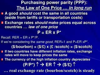
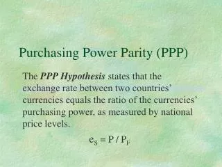
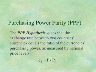
Purchasing Power Parity (PPP) Purchasing Power Parity (PPP) PPP is based on the law of one price (LOP): Goods, once denominated in the same currency, should have the same price. If they are not, then some form of arbitrage is possible. Example: LOP for Oil. Poil-USA = USD 80. Poil-SWIT = CHF 160. StLOP = USD 80 / CHF 160 = 0.50 USD/CHF. If St = 0.75 USD/CHF, then a barrel of oil in Switzerland is more expensive -once denominated in USD- than in the US: Poil-SWIT (USD) = CHF 160 x 0.75 USD/CHF = USD 120 > Poil-USA
Example (continuation): Traders will buy oil in the US (and export it to Switzerland) and sell the US oil in Switzerland. Then, at the end, traders will sell CHF/buy USD. This movement of oil from the U.S. to Switzerland will affect prices: Poil-USA↑; Poil-SWIT↓; & St↓ => StLOP↑ (St & StLOP converge) ¶ Note I: LOP gives an equilibrium exchange rate. Equilibrium will be reached when there is no trade in oil (because of pricing mistakes). That is, when the LOP holds for oil. Note II: LOP is telling what Stshould be (in equilibrium). It is not telling what Stis in the market today. Note III: Using the LOP we have generated a model for St. We’ll call this model, when applied to many goods, the PPP model.
Problem: There are many traded goods in the economy. Solution: Use baskets of goods. PPP: The price of a basket of goods should be the same across countries, once denominated in the same currency. That is, USD 1 should buy the same amounts of goods here (in the U.S.) or in Colombia.
• A popular basket: The CPI basket. In the US, the basket typically reported is the CPI-U, which represents the spending patterns of all urban consumers and urban wage earners and clerical workers. (87% of the total U.S. population). • U.S. basket weights:
• A potential problem with the CPI basket: The composition of the index (the weights and the composition of each category) may be very similar. • For example, the weight of the food category changes substantially as the income level increases.
Absolute version of PPP: The FX rate between two currencies is simply the ratio of the two countries' general price levels: StPPP = Domestic Price level / Foreign Price level = Pd / Pf Example: Law of one price for CPIs. CPI-basketUSA = PUSA = USD 755.3 CPI-basketSWIT = PSWIT = CHF 1241.2 StPPP= USD 755.3/CHF 1241.2 = 0.6085 USD/CHF. If St 0.6085 USD/CHF, there will be trade of the goods in the basket between Switzerland and US. Suppose St = 0.70 USD/CHF > StPPP. Then, PSWIT (in USD) = CHF 1241.2*0.70 USD/CHF = USD 868.70 > PUSA = USD 755.3
Example (continuation): PSWIT (in USD) = CHF 1241.2*0.70 USD/CHF = USD 868.70 > PUSA = USD 755.3 Potential profit: USD 868.70 – USD 755.3 = USD 93.40 Traders will do the following pseudo-arbitrage strategy: 1) Borrow USD 2) Buy the CPI-basket in the US 3) Sell the CPI-basket, purchased in the US, in Switzerland. 4) Sell the CHF/Buy USD 5) Repay the USD loan, keep the profits. ¶ Note: “Equilibrium forces” at work: 2) PUSA ↑ & 3) PSWIT ↓ (=> StPPP↑) 4) St ↓.
• Real v. Nominal Exchange Rates The absolute version of the PPP theory is expressed in terms of St, the nominal exchange rate. We can modify the absolute version of the PPP relationship in terms of the real exchange rate, Rt. That is, Rt= St Pf / Pd. Rt allows us to compare prices, translated to DC: If Rt> 1, foreign prices (translated to DC) are more expensive If Rt = 1, prices are equal in both countries –i.e., PPP holds! If Rt < 1, foreign prices are cheaper Economists associate Rt > 1 with a more efficient domestic economy.
Example: Suppose a basket –the Big Mac- cost in Switzerland and in the U.S. is CHF 6.23 and USD 3.58, respectively. Pf = CHF 6.23 Pd = USD 3.58 St = 1.012 USD/CHF => Pf = USD 6.3048 Rt= St PSWIT / PUS =1.012 USD/CHF x CHF 6.23/USD 3.58 = 1.7611. Taking the Big Mac as our basket, the U.S. is more competitive than Switzerland. Swiss prices are 76.11% higher than U.S. prices, after taking into account the nominal exchange rate. To bring the economy to equilibrium –no trade in Big Macs-, we expect the USD to appreciate against the CHF. According to PPP, the USD is undervalued against the CHF. => Trading signal: Buy USD/Sell CHF. 
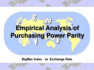
• The Big Mac (“Burgernomics,” popularized by The Economist) has become a popular basket for PPP calculations. Why? 1) It is a standardized, common basket: beef, cheese, onion, lettuce, bread, pickles and special sauce. It is sold in over 120 countries. Big Mac (Sydney) Big Mac (Tokyo) 2) It is very easy to find out the price. 3) It turns out, it is correlated with more complicated common baskets, like the PWT (Penn World Tables) based baskets. Using the CPI basket may not work well for absolute PPP. The CPI baskets can be substantially different. In theory, traders can exploit the price differentials in BMs.
• In the previous example, Swiss traders can import US BMs. From UH (US) to Rapperswill (CH) • This is not realistic. But, the components of a BM are internationally traded. The LOP suggests that prices of the components should be the same in all markets. The Economist reports the real exchange rate: Rt = StPBigMac,f/PBigMac,d. For example, for Norway’s crown (NOK): Rt = 7.02/3.58 = 1.9609 => (96.09% overvaluation)
Example: (The Economist’s) Big Mac Index Rt = StPBigMac,f/PBigMac,d (US=domestic)
• Empirical Evidence: Simple informal test: Test: If Absolute PPP holds => Rt= 1. In the Big Mac example, PPP does not hold for the majority of countries. Several tests of the absolute version have been performed: Absolute version of PPP, in general, fails (especially, in the short run). • Absolute PPP: Qualifications (1) PPP emphasizes only trade and price levels. Political/social factors (instability, wars), financial problems (debt crisis), etc. are ignored. (2) Implicit assumption: Absence of trade frictions (tariffs, quotas, transactions costs, taxes, etc.). Q: Realistic? On average, transportation costs add 7% to the price of U.S. imports of meat and 16% to the import price of vegetables. Many products are heavily protected, even in the U.S. For example, peanut imports are subject to a tariff as high as 163.8%. Also, in the U.S., tobacco usage and excise taxes add USD 5.85 per pack.
• Absolute PPP: Qualifications Some everyday goods protected in the U.S.: - European Roquefort Cheese, cured ham, mineral water (100%) - Paper Clips (as high as 126.94%) - Canned Tuna (as high as 35%) - Synthetic fabrics (32%) - Sneakers (48% on certain sneakers) - Japanese leather (40%) - Peanuts (shelled 131.8%, and unshelled 163.8%). - Brooms (quotas and/or tariff of up to 32%) - Chinese tires (35%) - Trucks (25%) & cars (2.5%) Some Japanese protected goods: - Rice (778%) - Beef (38.5%, but can jump to 50% depending on volume). - Sugar (328%) - Powdered Milk (218%)
• Absolute PPP: Qualifications (3) PPP is unlikely to hold if Pf and Pd represent different baskets. This is why the Big Mac is a popular choice. (4) Trade takes time (contracts, information problems, etc.) (5) Internationally non-traded (NT) goods –i.e. haircuts, home and car repairs, hotels, restaurants, medical services, real estate. The NT good sector is big: 50%-60% of GDP (big weight in CPI basket). Then, in countries where NT goods are relatively high, the CPI basket will also be relatively expensive. Thus, PPP will find these countries' currencies overvalued relative to currencies in low NT cost countries. Note: In the short-run, we will not take our cars to Mexico to be repaired, but in the long-run, resources (capital, labor) will move. We can think of the over-/under-valuation as an indicator of movement of resources.
• Absolute PPP: Qualifications The NT sector also has an effect on the price of traded goods. For example, rent and utilities costs affect the price of a Big Mac. (25% of Big Mac due to NT goods.) • Empirical Fact Price levels in richer countries are consistently higher than in poorer ones. This fact is called the Penn effect. Many explanations, the most popular: The Balassa-Samuelson (BS) effect. • Balassa-Samuelson effect. Labor costs affect all prices. We expect average prices to be cheaper in poor countries than in rich ones because labor costs are lower. This is the so-called Balassa-Samuelson effect: Rich countries have higher productivity and, thus, higher wages in the traded-goods sector than poor countries do. But, firms compete for workers. Then wages in NT goods and services are also higher =>Overall prices are lower in poor countries.
• For example, in 2000, a typical McDonald’s worker in the U.S. made USD 6.50/hour, while in China made USD 0.42/hour. • The Balassa-Samuelson effect implies a positive correlation between PPP exchange rates (overvaluation) and high productivity countries.
• Incorporating the Balassa-Samuelson effect into PPP: 1) Estimate a regression: Big Mac Prices against GDP per capita.
• Incorporating the Balassa-Samuelson effect into PPP: 2) Compute fitted Big Mac Prices (GDP-adjusted Big Mac Prices), along the regression (red) line. Use the difference between GDP-adjusted Big Mac Prices and actual prices (the white/blue dots) to estimate GDP-adjusted PPP over/under-valuation.
Relative PPP The rate of change in the prices of products should be similar when measured in a common currency (as long as trade frictions are unchanged): (Relative PPP) where, If = foreign inflation rate from t to t+T; Id = domestic inflation rate from t to t+T. Note: ef,TPPP is an expectation; what we expect to happen in equilibrium. • Linear approximation: ef,TPPP (Id - If) => one-to-one relation Example: From t=0 to t=1, prices increase 10% in Mexico relative to prices in Switzerland. Then, St should also increase 10%; say, from S0=9 MXN/CHF to S1=9.9 MXN/CHF. Suppose S1>9.9 MXN/CHF, then according to Relative PPP the CHF is overvalued. 
Example: Forecasting St (USD/ZAR) using PPP (ZAR=South Africa). It’s 2013. You have the following information: CPIUS,2013 = 104.5, CPISA,2013 = 100.0, S2011 =.2035 USD/ZAR. You are given the 2014 CPI’s forecast for the U.S. and SA: E[CPIUS,2014] = 110.8 E[CPISA,2014] = 102.5. You want to forecast S2014 using the relative (linearized) version of PPP. E[IUS-2014] = (110.8/104.5) - 1 = .06029 E[ISA-2014] = (102.5/100) - 1 = .025 E[S2014] = S2013 x (1 + ef,TPPP ) = S2013 x (1 + E[IUS]- E[ISA]) = .2035 USD/ZAR x (1 + .06029 - .025) = .2107 USD/ZAR.
Under the linear approximation, we have PPP Line Id - If PPP Line B (FC appreciates) A (FC depreciates) 45º ef,T (DC/FC) Look at point A: ef,T > Id - If, => Priced in FC, the domestic basket is cheaper => pseudo-arbitrage against foreign basket => FC depreciates
Relative PPP: Implications (1) Under relative PPP, Rt remains constant. (2) Relative PPP does not imply that St is easy to forecast. (3) Without relative price changes, an MNC faces no real operating FX risk (as long as the firm avoids fixed contracts denominated in FC). • Relative PPP: Absolute versus Relative - Absolute PPP compares price levels. Under Absolute PPP, prices are equalized across countries: "A mattress costs GBP 200 (= USD 320) in the U.K. and BRL 800 (=USD 320) in Brazil.“ - Relative PPP compares price changes. Under Relative PPP, exchange rates change by the same amount as the inflation rate differential (original prices can be different): “U.K. inflation was 2% while Brazilian inflation was 8%. Meanwhile, the BRL depreciated 6% against the GBP. Then, relative cost comparison remains the same.”
Relative PPP is a weaker condition than the absolute one. • Relative PPP: Testing Key: On average, what we expect to happen, ef,TPPP, should happen, ef,T. => On average: ef,T ef,TPPP Id – If or E[ef,T] = E[ef,TPPP] E[ Id – If ] A linear regression is a good framework to test theories. Recall, ef,T = (St+T - St)/St = α + β (Id - If )t+T + εt+T, where ε: regression error. That is, E[εt+T]=0. Then, E[ef,T] = α + β E[(Id - If )t+T] + E[εt+T] = α + β E[ef,TPPP ] =>E[ef,T] = α + β E[ef,TPPP ] • For Relative PPP to hold, on average, we need α=0 & β=1.
Relative PPP: General Evidence • Under Relative PPP:ef,T Id – If • 1. Visual Evidence • Plot (IJPY-IUSD) against st(JPY/USD), using monthly data 1970-2010. • Check to see if there is a No 45° line. No 45° line => Visual evidence rejects PPP.
2. Statistical Evidence More formal tests: Regression ef,T = (St+T - St)/St = α + β (Id - If )t+T + εt+T, -ε: regression error, E[εt+T]=0. The null hypothesis is: H0 (Relative PPP true): α=0 and β=1 H1 (Relative PPP not true): α≠0 and/or β≠1 • Tests: t-test (individual tests on α and β) and F-test (joint test) (1) t-test = [Estimated coeff. – Value of coeff. under H0]/S.E.(coeff.) t-test~ tv (v=N-K=degrees of freedom) (2) F-test = {[RSS(H0)-RSS(H1)]/J}/{RSS(H1)/(N-K)} F-test ~ FJ,N-K (J= # of restrictions in H0, K= # parameters in model, N= # of observations, RSS= Residuals Sum of Squared). • Rule: If |t-test| > |tv,α/2 |, reject at the α level. If F-test > FJ,N-K,α, reject at the α level. Usually, α = .05 (5 %)
Example: Using monthly Japanese and U.S. data (1/1971-9/2007), we fit the following regression: ef,t (JPY/USD) = (St - St-1)/St-1 = α + β (IJAP – IUS) t + εt. R2 = 0.00525 Standard Error (σ) = .0326 F-stat (slopes=0 –i.e., β=0) = 2.305399 (p-value=0.130) Observations (N) = 439 Coefficient Stand Err t-Stat P-value Intercept (α) 0.00246 0.001587 -1.55214 0.121352 (IJAP – IUS) (β)-0.36421 0.239873 -1.51835 0.129648 We will test the H0 (Relative PPP true): α=0 and β=1 Two tests: (1) t-tests (individual tests) (2) F-test (joint test)
Example: Using monthly Japanese and U.S. data (1/1971-9/2007), we fit the following regression: ef,t (JPY/USD) = (St - St-1)/St-1 = α + β (IJAP – IUS) t + εt. R2 = 0.00525 Standard Error (σ) = .0326 F-stat (slopes=0 –i.e., β=0) = 2.305399 (p-value=0.130) F-test (H0: α=0 and β=1): 16.289 (p-value: lower than 0.0001) => reject at 5% level (F2,467,.05= 3.015) Observations = 439 Coefficient Stand Err t-Stat P-value Intercept (α) -0.00246 0.001587 -1.55214 0.121352 (IJAP – IUS) (β) -0.36421 0.239873 -1.51835 0.129648 Test H0, using t-tests (t437.05=1.96 –Note: when N-K>30, t.05 = 1.96): tα=0: (-0.00246–0)/0.001587= -1.55214 (p-value=.12) => cannot reject tβ=1: (-0.36421-1)/0.239873= -5.6872 (p-value:.00001) => reject. 
• PPP Summary: - Short- run: PPP is a poor model to explain short-term St movements. - Long-run: Evidence of mean reversion for Rt. Currencies that consistently have high inflation rate differentials –i.e., (Id-If) positive-- tend to depreciate. • Let’s look at the MXN/USD case. We want to calculate StPPP= Pd,t / Pf,t over time. (1) Divide StPPP by SoPPP (t=0 is our starting point). (2) After some algebra, StPPP = SoPPP x [Pd,t / Pd,o] x [Pf,o/Pf,t] By assuming SoPPP = So, we plot StPPP over time. (Note: SoPPP = So assumes that at t=0, the economy was in equilibrium. This may not be true: Be careful when selecting a base year.)
Let’s look at the MXN/USD case. - In the short-run, StPPP is missing the target, St. - But, in the long-run, StPPP gets the trend right. (As predicted by PPP, the high Mexican inflation rates differentials against the U.S., depreciate the MXN against the USD.)
Another example, let’s look at the JPY/USD case. As predicted by PPP, since U.S. inflation rates have been consistently higher than the Japanese ones, in the long-run, the USD depreciates against the JPY.
• PPP Summary of Applications: - Equilibrium (“correct”) exchange rates. A CB can use StPPP to determine intervention bands. - Explanation of St movements(“currencies with high inflation rate differentials tend to depreciate”). - Indicator of competitiveness or under/over-valuation: Rt > 1 => FC is overvalued (& Foreign prices are not competitive). - International GDP comparisons: Instead of using St, StPPP is used. For example, per capita GDP (in 2012): Using market prices (St, actual exchange rates): U.S. GDP: USD 15.06 trillion, a 23.1% of the world’s GDP (27.5% in ’96). China’s GDP: USD 6.99 trillion, a 9.3% of the world’s GDP (3.1% in ’96). Under PPP exchange rates –i.e., StPPP: U.S. GDP: USD 15.06 trillion (the same) for a 20.0% share. China’s GDP: USD 11.3 trillion, for a 14.4% share.