
Understanding Contingency Tables and Probability Calculations with Visual Aid
This resource explores the concepts of contingency tables, tree diagrams, and the fundamentals of probability. By utilizing a full deck of cards as a case study, it illustrates how to calculate probabilities for various events, including the likelihood of drawing specific types of cards (e.g., red aces) and applying concepts such as joint and conditional probability. The text also covers key principles such as marginal probability, independence of events, and relevant formulas, making it an essential guide for understanding probabilistic outcomes in a systematic way.

Understanding Contingency Tables and Probability Calculations with Visual Aid
E N D
Presentation Transcript
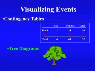
Visualizing Events • Contingency Tables • Tree Diagrams Ace Not Ace Total Black 2 24 26 Red 2 24 26 Total 4 48 52
Contingency Table A Deck of 52 Cards Red Ace Not an Ace Total Ace Red 2 24 26 Black 2 24 26 Total 4 48 52 Sample Space
Tree Diagram Event Possibilities Ace Red Cards Not an Ace Full Deck of Cards Ace Black Cards Not an Ace
Probability • Probabilityis the numerical • measure of the likelihood • that the event will occur. • Value is between 0and 1. • Sumof the probabilities of • all mutually exclusive • events is1. 1 Certain .5 0 Impossible
Computing Probability • The Probability of an Event, E: • Each of the Outcome in the Sample Space • equally likely to occur. e.g. P() = 2/36 (There are 2 ways to get one 6 and the other 4)
Joint Probability Using Contingency Table Event Total B1 B2 Event A1 P(A1andB1) P(A1andB2) P(A1) A2 P(A2 and B1) P(A2andB2) P(A2) 1 Total P(B1) P(B2) Marginal (Simple) Probability Joint Probability
Addition Rule P(A1or B1 ) = P(A1) +P(B1) - P(A1 andB1) Event Total B1 B2 Event A1 P(A1and B1) P(A1and B2) P(A1) P(A2 andB1) A2 P(A2 and B2) P(A2) 1 Total P(B1) P(B2) For Mutually Exclusive Events: P(A or B) = P(A) + P(B)
Dependent or Independent Events The Event of a Happy Face GIVEN it is Light Colored E = Happy Face ç Light Color 3 Items, 3 Happy Faces Given they are Light Colored
Computing Conditional Probability The Probability of the Event: EventAgiventhat EventBhas occurred P(A êB) = e.g. P(Red Card given that it is anAce) =
Conditional Probability Using Contingency Table Conditional Event: Draw 1 Card. Note Kind & Color Color Type Total Red Black Revised Sample Space 2 2 4 Ace 24 24 48 Non-Ace 26 26 52 Total
Conditional Probability and Statistical Independence Conditional Probability: P(AçB) = P(A and B) = P(AêB) • P(B) Multiplication Rule: Events are Independent: P(AêB) = P(A) Or, P(A and B) = P(A) • P(B) Events A and B are Independent when the probability of one event, A is not affected by another event, B.
Bayes’ Theorem:Contingency Table What are the chances of repaying a loan, given a college education? Loan Status Prob. Education Repay Default .2 .05 .25 College ? ? ? No College ? ? 1 Prob. ê P(RepayCollege) =
Discrete Probability Distribution • List ofAll Possible[ Xi, P(Xi) ]Pairs • Xi = Value of Random Variable (Outcome) • P(Xi) = Probability Associated with Value • Mutually Exclusive(No Overlap) • Collectively Exhaustive(Nothing Left Out) • 0 £P(Xi) £ 1 • SP(Xi) = 1
Binomial Probability Distributions • ‘n’ Identical Trials,e.g. 15 tosses of a coin, • 10 light bulbs taken from a warehouse • 2 Mutually Exclusive Outcomes, • e.g. heads or tails in each toss of a coin, • defective or not defective light bulbs • Constant Probabilityfor each Trial, • e.g. probability of getting a tail is the same each time we toss the coin and each light bulb has the same probability of being defective
Binomial Probability Distributions • 2 Sampling Methods: • Infinite Population Without Replacement • Finite Population With Replacement • Trials are Independent: • The Outcome of One Trial Does Not Affect the • Outcome of Another
Binomial Probability Distribution Function n ! X - X n P(X) = 1 ) p ( - p X ! ( - ) ! n X P(X) = probability that Xsuccesses given a knowledge of n and p X= number of ‘successes’ insample, (X = 0, 1, 2, ...,n) p = probability of ‘success’ n = sample size Tails in 2 Toss of Coin XP(X) 0 1/4 = .25 1 2/4 = .50 2 1/4 = .25
Binomial Distribution Characteristics n = 5p = 0.1 P(X) Mean .6 = E ( X ) = np m .4 .2 e.g. m=5 (.1) =.5 0 X 0 1 2 3 4 5 Standard Deviation n = 5p = 0.5 P(X) ) s = - p np ( 1 .6 .4 .2 e.g.s=5(.5)(1 - .5)= 1.118 X 0 0 1 2 3 4 5
P ( X = x | l - l x e l x ! Poisson Distribution • Poisson Process: • Discrete Eventsin an ‘Interval’ • The Probability ofOne Successin Interval is Stable • The Probability of More than One Success in this Interval is 0 • Probability of Success is • Independentfrom Interval to • Interval • e.g. # Customers Arriving in 15 min. • # Defects Per Case of Light Bulbs.
Poisson Probability Distribution Function -l X e l P ( X ) = X ! P(X ) = probability ofXsuccesses givenl l= expected (mean) number of ‘successes’ e = 2.71828 (base of natural logs) X = number of ‘successes’per unit e.g. Find the probability of4 customers arriving in 3 minutes when the mean is3.6. -3.6 4 e 3.6 P(X)= =.1912 4!
Poisson Distribution Characteristics Mean l = 0.5 P(X) .6 m = E ( X ) = l .4 N .2 å = 0 X X P ( X ) i i 0 1 2 3 4 5 i = 1 l = 6 P(X) .6 Standard Deviation .4 .2 s = l 0 X 0 2 4 6 8 10