4. Electronic structure of molecules
380 likes | 906 Vues
4. Electronic structure of molecules. . 4.1 The Schrödinger Equation for molecules 4.2 The Born-Oppenheimer approximation 4.3 Valence-bond theory 4.3.1 The hydrogen molecule 4.3.2 Polyatomic molecules 4.3.3 Hybridization 4.4. Molecular orbital theory 4.4.1 The hydrogen molecule-ion

4. Electronic structure of molecules
E N D
Presentation Transcript
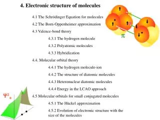
4. Electronic structure of molecules 4.1 The Schrödinger Equation for molecules 4.2 The Born-Oppenheimer approximation 4.3 Valence-bond theory 4.3.1 The hydrogen molecule 4.3.2 Polyatomic molecules 4.3.3 Hybridization 4.4. Molecular orbital theory 4.4.1 The hydrogen molecule-ion 4.4.2 The structure of diatomic molecules 4.4.3 Heteronuclear diatomic molecules 4.4.4 Energy in the LCAO approach 4.5 Molecular orbitals for small conjugated molecules 4.5.1 The Hückel approximation 4.5.2 Evolution of electronic structure with the size of the molecules 2+
4.1 The Schrödinger Equation for molecules All properties of a molecule (= M nuclei + n electrons) can be evaluated if we find the wavefunction (x1, x2,..., xn) by solving the Schrödinger equation (SE): H =E. H= Ttot + Vtot= (TN + Te )+ (VeN + Vee + VNN) The total kinetic operator of the molecule is composed of a part for the nuclei TN and one for the electrons Te. The total potential energy operator is the sum of the electron/electron (Vee), electron/nucleus (VeN) and nucleus/nucleus (VNN) interactions. Rj are the nucleus coordinates and ri the electronic coordinates. Mj is the mass of the nucleus j and mi is the electron mass. Zj is the number of protons in the nucleus j and e is the charge of an electron. Solving with the best approximation the SE is the challenge of quantum chemistry (W. Kohn and J. Pople: Nobel Prize in Chemistry 1998). In this chapter, we introduce the vocabulary and the basic principles to understand the electronic structure of molecules.
4.2 The Born-Oppenheimer approximation The electrons are much lighter than the nuclei (me/mH1/1836) →their motion is much faster than the vibrational and rotational motions of the nuclei within the molecule. A good approximation is to neglect the coupling terms between the motion of the electrons and the nuclei: this is the Born-Oppenheimer approximation. The Schrödinger equation can then be divided into two equations: 1) One describes the motion of the nuclei. The eigenvalues of this nuclear part of the SE gives the discrete energetic levels of the vibration and rotation of the molecule. → see Chap 6: the vibrational spectroscopy is used to observed transition between these energetic levels. 2) The other one describes the motion of the electrons around the nuclei whose positions are fixed. This electronic part of the SE is the “electronic Schrödinger equation”: → The knowledge of the electronic wavefunction is necessary to understand chemical bonding, electronic and optical properties of the matter. In the rest of the chapter, we’ll only speak about electronic wavefunction.
D0 The electronic Schrödinger equation The nuclear coordinate R appears as a parameter in the expression of the electronic wave function. An electronic wave function elect(R,r) and an energy Eelectare associated to each structure of the molecule (set of nuclei coordinates R). For each variation of bond length in the molecule (each new R), the electronic SE can be solved and the energy that the molecule would have in this structure can be estimated: the molecular potential energy curve is obtained (see Figure). The molecule is the most stable (minimum of energy) for one specific position of the nuclei: the equilibrium position Re. R The zero energy corresponds to the dissociated molecule. The depth of the minimum, De, gives the bond dissociation energy, D0, considering the fact that vibrational energy is never zero, but ½ħ : D0=De- ½ħ
4.3 Valence-bond theory 4.3.1 The hydrogen molecule A(1) = H1sA(r1) is the wavefunction of the electron 1 on the 1s orbital of Hydrogen A. When the atoms are close, it’s not possible to know whether it is electron 1 that is on A or electron 2. += A(1)B(2) +A(2)B(1) The system is described by a superposition of the wavefunctions for each possibility: A(1)B(2) and A(2)B(1). Two linear combinations are possible: -= A(1)B(2) -A(2)B(1) += A(1)B(2) + A(2)B(1)→ between the two nuclei: |+|2>0 creation of a bond described by a “bonding molecular orbital”: stabilization of the 2-H system. -= A(1)B(2) -A(2)B(1)→ between the two nuclei, - changes sign → |-|2 =0 →creation of a * bond described by a “antibonding molecular orbital”.
What is the spin of the 2 electrons involved in the bond? The total electronic wavefunction (x1,x2) of H2 must be antisymmetric. The spatial orbital forming the bond is symmetric → the spin function S(1,2) should be antisymmetric (see Chap 3). The only antisymmetric spinfunction for a system of 2 e- corresponds to antiparallel spins. (1,2)= +(1,2) S(1,2)= 1/21/2 [A(1)B(2) + A(2)B(1)]{(1)(2) - (1)(2)} The spatial orbital +(1,2) gives an energy for the 2-H system that is lower than the energy of 2 Hydrogen atoms far from each other: bond formation. The spinfunction corresponding to this stable situation shows that the spins are paired. The formation of a bond is achieved if the electron spins are paired
y z x 4.3.2 Homonuclear diatomic molecules N 1s2 2s2 2px1 2py1 2pz1 Valence electrons In N2: 3 bonds are formed by combining the 3 different 2p orbitals of the 2 nitrogen atoms. This is possible because of the symmetry and the position of those 2p orbitals with respect to each other. one bond and 2 bonds (perpendicular to each other) are formed by spin pairing.
4.3.3 Polyatomic molecules O 1s2 2s2 2px2 2py1 2pz1 x H 1s1 H 1s1 y z H2O: This simple model suggests that the formed angle between the (O-H) bonds is 90°, as well as their position vs. the paired 2px electrons; whereas the actual bond angle is 104.5°.
A. Promotion C: 1s2 2s2 2px1 2py1. With the valence bond theory, we expect maximum 2 bonds. But, tetravalent carbon atoms are well known: e.g., CH4. This deficiency of the theory is artificially overcome by allowing for promotion. Promotion:the excitation of an electron to an orbital of higher energy. This is not what happens physically during bond formation, but it allows to feel the energetics. Indeed, following this artificial excitation, the atom is allowed to create bonds; and consequently, the energy is stabilized… more than the cost of the excitation energy. C: 1s2 2s2 2px1 2py1→ 1s2 2s1 2px1 2py1 2pz1. CH4 should be composed of 3 bonds due to the overlap between the 2p of C and the 1s of H, and another bond coming from the 2s of C and the 1s of H. But, it is known that CH4 has 4 similar bonds. This problem is overcome by realizing that the wavefunction of the promoted atom can be described on different orthonormal basis sets: 1) either the orthogonal hydrogenoic atomic orbitals (AO): 1s, 2s, 2px, 2py, 2pz. 2) or equivalently, from another set of orthonormal functions: “the hybrid orbitals”
B. Hybridization sp3 h1= s + px + py+ pz h2= s - px + py- pz h3= s - px - py+ pz h4= s + px - py- pz An orthonormal set of hybrid orbitals is created by applying a transformation on the orthonormal hydrogenic orbitals. The sp3, sp2 or sp hybrid orbitals are linear combinations of the AO’s, they appear as the resulting interference between s and p orbitals. sp3 hybridization + - Each hybrid orbital has the same energy and can be occupied by one electron of the promoted atom CH4 has 4 similar bonds.
H H H H sp2 hybridization hi The sp2 hybrid orbitals lie in a plane and points towards the corners of an equilateral triangle. 2pz is not involved in the hybridization, and its axis is perpendicular to the plane of the triangle. h1= s +21/2 py h2= s + (3/2)1/2 px - (1/2)1/2 py h3= s - (3/2)1/2 px - (1/2)1/2 py 120° An hybrid orbital has pronounced directional character because it has enhanced amplitude in the internuclear region, coming from the constructive resulting interference. Consequently, the bond formation is accompanied with a high stability gain. 2pz In ethene CH2=CH2, the hybrid orbitals of each C atom create the backbone of the molecule via 3 bonds (2 C-H and 2 C-C). The remaining 2pz of the 2 C atoms create a bond preventing internal rotation.
x y z H Nu C X H H sp hybridization In ethyne, HC≡CH: Formation of 2 bonds (with C and H) using the 2 hybrid orbitals h1 and h2. The remaining 2px and 2py can form two bonds between the two carbon atoms. h1= s + pz h2= s - pz Other possible hybridization ? Note: 'Frozen' transition states: pentavalent carbon et al ; Martin-JC; Science.vol.221, no.4610; 5 Aug. 1983; p.509-14. Organic ligands have been designed for the stabilization of specific geometries of compounds of nonmetallic elements. These ligands have made possible the isolation, or direct observation, of large numbers of trigonal bipyramidal organo-nonmetallic species. Many of these species are analogs of transition states for nucleophilic displacement reactions and have been stabilized by the ligands to such a degree that they have become ground-state energy minima. Ideas derived from research on these species have been applied to carbon species to generate a molecule that is an analog of the transition state for the associative nucleophilic displacement reaction. The molecule is a pentavalent carbon species that has been observed by nuclear magnetic resonance spectroscopy. Sketch of the transition state species during a nucleophilic substitution SN2 CH3X + Nu-→CH3Nu + X-
e- rA rB R A B 4.4. Molecular orbital (MO) theory 4.4.1 The hydrogen molecule-ion: H-H+ A. Linear combination of atomic orbitals (LCAO) The electron can be found in an atomic orbital (AO) belonging to atom A (i.e.; 1s of H) and also in an atomic orbital belonging to B (i.e.; 1s of H+) The total wavefunction should be a superposition of the 2 AO and it is called molecular orbital LCAO-MO. Let’s write the atomic orbitals on the two atoms by the letters A and B. ±= N(A ± B) N is the normalization constant. Example for += N(A + B): is the overlap integral related to the overlap of the 2 AO
+ B. Bonding orbitals The LCAO-MO: += {2(1+S)}-1/2(A + B), with A=1s, B=1s of H Probability density: 2+= {2(1+S)}-1(A2 + B2 + 2AB) A2 = probability density to find the e- in the atomic orbital A B2 = probability density to find the e- in the atomic orbital B 2AB = the overlap density represents an enhancement of the probability density to find the e- in the internuclear region: the electron accumulates in regions where AO’s overlap and interfere constructively; which creates a bonding orbital 1 with one electron. 2+ C. Antibonding orbitals - -= {2(1-S)}-1/2(A - B) Probability density: 2-= {2(1-S)}-1(A2 + B2 - 2AB) -2AB = reduction of the probability density to find the e- in the internuclear region: there is a destructive interference where the two AO overlap, which creates an antibonding orbital *. Nodal plane between the 2 nuclei 2-
D. Energy of the states and * e- rA rB R A B H-H+: One electron around 2 protons += {2(1+S)}-1/2(A + B) =- H = E -= {2(1-S)}-1/2(A - B) =+ j= measure of the interaction between a nucleus and the electron density centered on the other nucleus k= measure of the interaction between a nucleus and the excess probability in the internuclear region S= measure of the overlap between 2 AO. S decreases when R increases. Note: S=0 for 2 orthogonal AO.
4.4.2 Structure of diatomic molecules Now, we use the molecular orbitals (= + and *= -) found for the one-electron molecule H-H+; in order to describe many-electron diatomic molecules. A. The hydrogen and helium molecules H2: 2 electrons ground-state configuration: 12 E Increase of electron density He2: 4 electrons ground-state configuration: 12 2*2 E E- E+<E- He2 is not stable and does not exist E+
B. Bond order n= number of electrons in the bonding orbital n*= number of electrons in the antibonding orbital Bond order:b=½(n-n*) The greater the bond order between atoms of a given pair of elements, the shorter is the bond and the greater is the bond strength. C. Period 2 diatomic molecules According to molecular orbital theory, orbitals are built from all orbitals that have the appropriate symmetry. In homonuclear diatomic molecules of Period 2, that means that two 2s and two 2pz orbitals should be used. From these four orbitals, four molecular orbitals can be built: 1, 2*, 3, 4*. 1, 2*, 3, 4*. With N atomic orbitals the molecule will have N molecular orbitals, which are combinations of the N atomic orbitals.
dioxygen O2: 12 valence electrons The two last e- occupy both the x* and the y* in order to decrease their repulsion. The more stable state for 2e- in different orbitals is a triplet state. O2 has total spin S=1 (paramagnetic) (see Chap 3) The two 2px give one x and one x* The two 2py give one y and one y* Bond order = 2
4.4.3 Heteronuclear diatomic molecules A diatomic molecule with different atoms can lead to polar bond, a covalent bond in which the electron pair is shared unequally by the 2 atoms. A. Polar bonds 2 electrons in an molecular orbital composed of one atomic orbital of each atom (A and B). = cA A + cB B |ci|2= proportion of the atomic orbital “i” in the bond The situation of covalent polar bonds is between 2 limit cases: 1) The nonpolar bond (e.g.; the homonuclear diatomic molecule): |cA|2= |cB|2 2) The ionic bond in A+B- : |cA|2= 0 and |cB|2=1 Example: HF The H1s electron is at higher energy than the F2p orbital. The bond formation is accompanied with a significant partial negative charge transfer from H to F.
B. Electronegativity A measure of the power of an atom to attract electron to itself when it is part of a compound. There are different electronegativity definitions, e.g. the Mulliken electronegativity: M=½ (IP + EA) IP is the ionization potential = the minimum energy to remove an electron from the ground state of the molecule (Chap 3, p14). EA is the electron affinity = energy released when an electron is added to a molecule. EA>0 when the addition of the electron releases energy, i.e. when it stabilizes the molecule.
C. Variation principle All the properties of a molecule can be found if the wavefunction is known: e.g., the electron density distribution or the partial atomic charge. The wavefunction can be found by solving the Schrödinger equation…. But the latter is impossible to solve analytically!! We use the variation principle to go around that problem and find approximate wavefunction. The variation principle is the basic principle to determine wavefunction of complicated molecular systems. The idea is to optimize the coefficient cA and cB of the wavefunction, =cAA + cBB, such that the system is the most stable, i.e. the energy is minimal. Variation principle: “If an arbitrary wavefunction is used to calculate the energy, the value calculated is never less than the true energy.” In the end of the chapter, we’ll try to find the best coefficients cito give to the trial wavefunction in order to approach the true energy. More sophisticated methods: (i) increase the set of atomic orbitals, called “the basis set” from which the molecular orbital is expressed; (ii) improve the description of the system by using more correct Hamiltonian H. (cA, cB) =cAA + cBB H=E E >Etrue Aim: Try to find the (cA, cB) that minimize the calculated E
4.4.4 Energy in the LCAO approach (1) Numerator: A is a Coulomb integral: it is related to the energy of the e- when it occupies A. ( < 0) is a Resonance integral: it is zero if the orbital don’t overlap. (at Re, <0) (1) Denominator: (1)
Let’s find the coefficients cA and cB: cA should minimize E: Secular equations cB should minimize E: See next page In order to have a solution, other than the simple solution cA= cB= 0, we must have: Secular determinant should be zero The 2 roots give the energies of the bonding and antibonding molecular orbitals formed from the AOs
D. Homonuclear diatomic molecules 1) : =cAA + cBB with A= B →A= B= (1) (2) bonding (1) (2) antibonding 0 antibonding= {2(1-S)}-1/2(A - B) bonding= {2(1+S)}-1/2(A + B)
0 Eantibonding= - E- Ebonding = E+- Since: 0 < S < 1 Eantibonding > Ebonding Note 1: He2 has 4 electrons ground-state configuration: 12 2*2 He2 is not stable! Note 2: If we neglect the overlap integral (S=0), Eantibonding = Ebonding= The resonance integral is an indicator of the strength of covalent bonds
4.5. Molecular orbitals of small conjugated molecules 4.5.1 The Hückel approximation Here, we investigate conjugated molecules in which there is an alternation of single and double bonds along a chain of carbon atoms. In the Hückel approach, the orbitals are treated separately from the orbitals, the latter form a rigid framework that determine the general shape of the molecule. All C are considered similar → only one type of coulomb integral for the C2p atomic orbitals involved in the molecular orbitals spread over the molecule. A. The secular determinant The molecular orbitals are expressed as linear combinations of C2pz atomic orbitals (LCAO), which are perpendicular to the molecular plane. Ethene, CH2=CH2: =cAA + cBB, where A and B are the C2pz orbitals of each carbon atoms. Butadiene, CH2=CH-CH=CH2: =cAA + cBB+ccC + cDD The coefficients can be optimized by the same procedure described before: express the total energy E as a function of the ci and then minimize the E with respect to those coefficients ci. Inject the energy solutions in the secular equations and extract the coefficients minimizing E.
i 2pz i+2 i+1 Following these methods and since A= B= , we obtain those secular determinants: Ethene, CH2=CH2: Butadiene, CH2=CH-CH=CH2: Hückel approximation: 1) All overlap integrals Sij= 0 (ij). 2) All resonance integrals between non-neighbors, i,i+n=0 with n 2 3) All resonance integrals between neighbors are equal, i,i+1= i+1,i+2 = Severe approximation, but it allows us to calculate the general picture of the molecular orbital energy levels.
B. Ethene and frontier orbitals Within the Hückel approximation, the secular determinant becomes: E- = - energy of theLowest Unoccupied Molecular Orbital (LUMO) E+ = + energy of theHighest Occupied Molecular Orbital (HOMO) LUMO= 2* 2|| HOMO= 1 HOMO and LUMO are the frontier orbitals of a molecule. those are important orbitals because they are largely responsible for many chemical and optical properties of the molecule. Note: The energy needed to excite electronically the molecule, from the ground state 12 to the first excited state 11 2*1is provided roughly by 2|| ( is often around -0.8 eV) Chap 7
Ethene ethene deshydrogenation nickel Ethyne http://www.fhi-berlin.mpg.de/th/personal/hermann/pictures.html
4.5.2 Evolution of electronic structure with the size of the molecules A. Butadiene and delocalization energy 4th order polynomial 4 roots E There is 1e- in each 2pz orbital of the four carbon atoms 4 electrons to accommodate in the 4 -type molecular orbitals the ground state configuration is 12 22 The greater the number of internuclear nodes, the higher the energy of the orbital Butadiene C4H6: total -electron binding energy, E isE = 2E1+2E2= 4 + 4.48 with two -bonds Ethene C2H4:E = 2 + 2 with one -bond Two ethene molecules give: E = 4 + 4 for two separated -bonds. The energy of the butadiene molecule with two -bonds lies lower by 0.48 (-36kJ/mol) than the sum of two individual -bonds: this extra-stabilization of a conjugated system is called the “delocalization energy” 3 nodes = E4 2 nodes = E3 LUMO= 3* = E2 1 node HOMO= 1 = E1 0 node Top view of the MOs
D. Benzene and aromatic stability Scheme of the different orbital overlaps Each C has: - 3 electrons in (sp2) hybrid orbitals 3 bonds per C - 1 electron in 2pz one bond per C 6* E6 = - 2 6 electrons 2pz to accommodate in the 6 -molecular orbitals the ground state configuration is 12 22 32. E4,5= - 4* Benzene C6H6: total -electron binding energy, E is E = 2E1+4E2= 6 + 8 with three -bonds Three ethene molecules give: E = 6 + 6 for 3 separated -bonds. The delocalization energy is 2 (-150kJ/mol) 5* E2,3 = + 2 3 E1 = + 2 1
Benzene C6H6 is more stable than the hexatriene. Both molecules has 3 -bonds, but the cyclic structure of benzene stabilizes even more the -electrons. The symmetry of benzene creates two degenerated -bonds (2 and 3). When they are occupied, this is a more stable situation than the 12 22 32 configuration for hexatriene aromatic stability 6* 4* 5* 3 2 3 2 1 1