Download

1 / 46
610 likes | 1.7k Vues
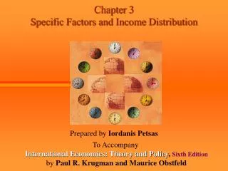
Lectures 4-5: The specific factors model. Giovanni Facchini. Outline. Introduction The specific factors model International trade in the specific factors model Income distribution and the gains from trade The political economy of international trade policy Summary. Introduction.

E N D
Lectures 4-5: The specific factors model Giovanni Facchini
Outline • Introduction • The specific factors model • International trade in the specific factors model • Income distribution and the gains from trade • The political economy of international trade policy • Summary
Introduction • International trade has important income distribution consequences within a country. • There are two fundamental reasons for why trade has important effects on income distribution: • Production factors cannot instantaneously relocate from one sector to another at zero cost. • Factor’s demand vary by sector. • The specific factors model highlights how trade affects the income distribution.
The specific factors model • Assumptions • The economy produces two goods, manufactured goods (M) and food (F) • There are three production factors : labor (L), capital (K) and land (T). • Manufactured goods are produced using capital and labor (but not land). • Food is produced using land and labor (but not capital). • Thus labor is mobile because it is used by both sectors • Land and capital are specific factors that can be used in the production of one good only. • All markets are perfectly competitive.
The specific factors model • How much of each good is produced? • The production of manufactured goods depends on the quantity of labor and capital used in the sector. • This relationship is captured by the production function. • The production function for good X characterizes the maximum quantity of good X that can be produced using all possible combinations of factors. • For example, the production function for manufactured goods (food) tells us the quantity of manufactured goods (food) that we can produce for any given quantity of capital (land) and labor.
The specific factors model • The production function for manufactured goods is given by QM = QM (K, LM) (3-1) where: • QM is the output of manufactured goods • K is the endowment of capital • LMis the number of workers employed in the M sector • The production function for manufactured goods is given by QF = QF (T, LF) (3-2) where: • QF is the output of food • T is the endowment of land • LF is the number of workers employed in the F sector
The specific factors model • The labor market equilibrium under full employment implies that: LM + LF = L(3-3) • We can use these relationships to construct the production possibility frontier of the country.
The specific factors model • The production possibility frontier • To analyze the production possibility frontier of the country we need to ask how the output mix of the country varies as labor relocates from one sector to the other. • Figure 1 shows the production function for manufactured goods.
QM QM = QM(K, LM) LM The specific factors model Figure 1: The manufactured goods production function
The specific factors model • The shape of the production function highlights the presence of decreasing marginal product of labor • Adding an extra worker to the production process, keeping capital constant, implies a reduction in the quantity of capital per worker. • Therefore, every additional unit of labor will imply an increase in output at a decreasing rate. • Figure 2 depicts the marginal productivity of labor, i.e. the increase of output brought about by an additional unit of labor.
MPLM MPLM LM The specific factors model Figure 2: The marginal product of labor
QF (increasing ) 1' 2' QF =QF(K, LF) Q2F 3' L2F PP QM (increasing ) LF(increasing) L Q2M L2M 1 2 3 L AA LM (increasing ) QM =QM(K, LM) The specific factors model Figure 3: The PPF in the specific factors model Food production function Production possibility frontier(PP) Manufactured goods production function Labor allocation(AA)
Slope of the PP curve • Ricardian model: • The PP curve is a straight line because the opportunity cost of food in terms of manufacturing is constant • Specific factors model: • The PP curve illustrates the presence of decreasing marginal productivity of labor in each sector. The slope is given by - MPLF /MPLM • To increase the ooutput of manufactured goods by one unit, the economy needs to reduce the output of food by MPLF /MPLM
The specific factors model • Prices, wages and labor allocation • How much labor will be used by each sector? • To answer this question, we need to consider the demand and the supply of labor. • Labor demand: • In each sector, employers will try to maximize profits, hiring workers up to the point in which the marginal product of labor is equal to the cost of hiring that additional unit.
The firm’s problem • In each sector, the firm maximizes profits, i.e. it solves the following problem and the corresponding first order condition is given by
The specific factors model • The labor demand curve in the manufacturing sector is given by MPLMxPM = w • The wage is equal to the value of the marginal product in the manufacturing sector. • The labor demand in the food sector is instead given by: MPLF xPF = w • Once again, the wage is equal to the value of the marginal product in the manufacturing sector.
The specific factors model • In equilibrium, the salary has to be the same in the two sectors, as a result of the perfect mobility of labor. • The wage is determined as a result of market clearing: LM + LF = L
W W PFX MPLF (Labor demand in the food sector) 1 W1 PMX MPLM (Labor demand in the manufacturing sector) Labor employed in the manufacturing sector,LM Labor employed in the food sector , LF L1M L1F Overall labor supply L The specific factors model The allocation of labor between sectors
Labor demand in the food sector • In equilibrium, the PPF is tangent to the line whose slope is given by the relative price of manufacturing in terms of food (with a minus sign). • The relationship between relative prices and output levels is given by : -MPLF/MPLM = -PM/PF
QF 1 Q1F PP QM Q1M The specific factors model Figure 5: Output in the specific factors model Slope = -(PM/PF)1
The specific factors model • What happens to the allocation of labor and the income distribution if the price of food and the price of the manufactured goods change? • Two possible scenarios: • Proportional variation in prices • Change in relative prices
PF2 X MPLF W PM2X MPLM W PM1 X MPLM 2 W2 PF1 X MPLF 1 W1 Labor employed in the manufacturing sector LM Labor employed in the Food sector, LF The specific factors model Proportional increase in the two prices PM increases by 10% PF increases by 10% Increase by 10% in the salary
The specific factors model • When prices change by the same proportion, there is no effect in real terms. • The wage (w) increases proportionally with the prices, and as a result real wages are unaffected. • The capital- and land- owners real incomes are also unaffected.
The specific factors model • If only PM increases, labor relocates from the food to the manufacturing sector and the output level increases in the manufacturing sector, while it decreases in the food sector. • The wage (w) does not increase as much as PM, since employment in the manufacturing sector increases and thus the marginal productivity of labor in that sector decreases.
W W PF1X MPLF 2 Increase in the wage by less than 10% W 2 1 PM2X MPLM W1 PM1X MPLM Labor employed in the manufacturing sector Labor employed in the Food sector Quantity of labor Relocating to manufacturing The specific factors model An increase in the price of manufacturing by 10% Increase in the relative demand by 10%
QF Q1F 1 Q2F 2 PP Q2M QM Q1M The specific factors model Figure 8: The effect of a change in the relative price of manufacturing Solpe= - (PM/PF)1 Slope= - (PM /PF) 2
The specific factors model • Relative prices and income distribution • Assume that PM increases by 10%. Then, we expect an increase in wages by less than 10%, for example 5%. • What is the effect of this increase on the income of the following three groups? • Workers • Capital owners • Landowners
The specific factors model • Workers: • The effect is indeterminate. It depends on the relative importance of the consumption of the two goods. • Capital owners: • They are better off. The inflow of additional workers in the manufacturing sector increases the marginal productivity of capital. • Land owners: • They are worse off. The outflow of workers from the food sector decreases the marginal productivity of land.
RS 1 (PM /PF)1 RD (QM /QF)1 The specific factors model Figure 9: Determining relative prices PM/PF QM/QF
International trade in the specific factors model • Assumptions: • Assume that both countries (say Japan and the US) share the same preferences and thus the same relative demand. • Thus the only source of trade is represented by differences in the relative supply across countries. The relative supply might differ because of • technology • different endowments of production factors (capital, labor, land) • We will assume that there are differences in factor endowments.
International trade in the specific factors model • Endowments and relative supply • What are the effects of an increase in the capital endowment on the output of manufactured goods and food? • A country with a large endowment of capital will produce a higher ratio of manufacturing to food for every given combination of relative prices.
International trade in the specific factors model W W PF1 X MPLF 2 W2 1 W1 PMX MPLM2 PMX MPLM1 Labor employed in the Food sector Labor relocating to the manufacturing sector Labor employed in the manufacturing sector Figure 10: An increase in the endowment of capital Increase in the capital stock K
International trade in the specific factors model • An increase in the endowment of capital leads to a shift to the right of the relative supply • An increase in the endowment of land leads to a shift to the left of the relative supply • What happens if the labor supply increases? • The effect on the relative output level is ambiguous, even though we know that both outputs will increase.
International trade in the specific factors model • International trade and relative prices • Assume that Japan (J) has more capital per worker than the USA (A). Analogously, the USA have more land per worker than Japan. • As a result, the relative price of manufactured goods in autarky is lower in Japan than in the USA. • International trade brings about a convergence in relative prices.
International trade in the specific factors model. PM /PF RSA RSWORLD (PM/PF )A RSJ (PM /PF )W (PM/PF)J RDWORLD QM/QF Figure 11: International trade and relative prices
International trade in the specific factors model. • The structure of trade flows • In autarky, production must be equal to consumption • If trade is possible, the combinations of manufactured goods and food that are consumed might differ from those that are produced. • Still, a country cannot spend more than the value of its output (no borrowing in this model).
International trade in the specific factors model. Food Consumption, DF Food Production, QF 1 Q1F PPF Manufactured consumption, DM Manufactured production, QM Q1M Figure 12: The budget constraint of a trading economy Budget constraint (slope = -PM/PF)
International trade in the specific factors model F F US food exports J’s food imports M M QJM QAM DJM DAM J’s manufactured goods exports US food imports Figure 13: Equilibrium under free trade US budget constraint Japan’s budget constraint QAF DAF DJF QJF
Income distribution and the gains from international trade • To assess the effect of trade on income distribution, we need to remember that international trade changes the relative good prices . • International trade improves the welfare of the specific factor used in the sector producing export goods, but it reduces the welfare of the specific factor used in the production of import competing goods. • International trade has an ambiguous effect on the mobile factor.
Income distribution and the gains from international trade • It is possible for those who gains from international trade to compensate those who lose from it? • If this is the case, international trade is potentially Pareto improving, i.e. it can make everybody better off. • International trade increases overall welfare because it expands the consumption possibility set. • The expansion of the consumption possibility set implies that everybody can – potentially at least – be made better off as a result of international trade.
Food consumption, DF Food production, QF 2 1 Budget constraint (slope = - PM/PF) Q1F PP Q1M Manuf. consumption, DM Manuf. production, QM Income distribution and the gains from international trade Figure 14: International trade expands the consumption possibilities of each country
The political economy of trade policy: a preliminary look • International trade creates winners and losers. • The optimal trade policy • The government needs to trade off the gains of some groups against the losses of some other groups • Some groups ask for protection because they are already poor (for examples, US workers in the shoe, apparel industries). • Most economists are still in favor of open trade policies. • To understand how trade policies come about, we need to understand the true reasons behind trade policy choices.
The political economy of trade policy: a preliminary look • Income distribution and trade policies • Usually, those who gain from trade are much less informed than thos who lose from trade. • Example: sugar producers and consumers in the United States.
Summary • International trade has important effects on the income distribution within a country, thus creating winners and losers • Income distribution effects are due to: • Production factors cannot relocate costlessly between one sector and the other. • Changes in the output mix have different effects on the demand for production factors.
Summary • The specific factors model is a useful tool in the analysis of the income distribution effects of trade • In this model, differences in factor endowments might lead to differences in the relative supply curves and thus lead to international trade. • In each country, specific factors used in the exporting sectors benefit from opening up trade, while the specific factors used in the import competing sectors lose. • The mobile factor, which is used in both sectors, might gain or lose..
Summary • International trade brings about aggregate gains, which can be used – at least as a matter of principle – to compensate the losers, and thus bring about Pareto gains from trade.