Download
1 / 54
550 likes | 724 Vues
The Supply Side of The Market. Inputs used in production LABOR CAPITAL Land Energy Output Raw materials Human knowledge Information Entrepreneurship. Main factors of production. Total production: Q = f( L , K ) Marginal product: Average product:.

E N D
The Supply Side of The Market
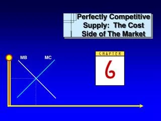
Inputs used in production • LABOR • CAPITAL • Land • Energy Output • Raw materials • Human knowledge • Information • Entrepreneurship Chapter 6: Perfectly Competitive Supply
Main factors of production • Total production: Q = f(L, K) • Marginal product: • Average product: Chapter 6: Perfectly Competitive Supply
Profit-Maximizing Firms in Perfectly Competitive Markets • Concepts of production • Fixed factor of production • An input whose quantity cannot be altered in the short run • Variable factor of production • An input whose quantity can be altered in the short run In economics, we assume K is fixed and L is variable in the short run. All factors of production are variable in the long run. Chapter 6: Perfectly Competitive Supply
Q Q = f(L) Q1 Production set L L1 Law of Diminishing Returns • Production function: the maximum output with a given level of Labor, holding Capital constant Chapter 6: Perfectly Competitive Supply
Important Cost Concepts Fixed costs • Costs paid at the beginning (to enable production), that you must bear even if you don’t produce. • Fixed costs do not vary with Q. • Fixed costs are sunk cost once they are paid. Examples: buying a photocopy machine to start-up a photocopy shop, renting a photocopy machine for 1 year, building a factory. Chapter 6: Perfectly Competitive Supply
Important Cost Concepts • Variable cost • Costs, which are proportional to Q. In other words, costs that occur with each unit produced; such as raw material input or labor. For example, salary paid to the operator of the photocopy machine, paper, ink, electricity consumption. Chapter 6: Perfectly Competitive Supply
Important Cost Concepts • Total Cost = Fixed cost + variable cost • Marginal Cost • Measures how total cost changes with a one-unit change in output Chapter 6: Perfectly Competitive Supply
Profit-Maximizing Firms in Perfectly Competitive Markets • Average Variable Cost and Average Total Cost • Average Variable Cost • Variable cost divided by total output • Average Total Cost • Total cost divided by total output Chapter 6: Perfectly Competitive Supply
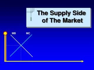
C MC(q) AC(q) AVC(q) q Average and marginal costs • Average and marginal cost curves must intersect at the minimum point of average cost Chapter 6: Perfectly Competitive Supply
Average and marginal costs (2) If MC(q) < AC(q), AC(q) must decrease If MC(q) > AC(q), then AC(q) must increase Conclusion: MC(q) and AC(q) can only intersect if MC(q) = AC(q) Example: the firm’s cost function: At what price will this firm break-even? P = AC(q) and P = MC(q), thus AC(q) = MC(q) Chapter 6: Perfectly Competitive Supply Slide 11
Average Variable Cost and Average Total Cost of Bottle Production Average total cost ($/unit of output) Average variable cost ($/unit of output) Average Variable cost ($/bottle) Variable cost ($/day) Total cost ($/day) Employees per day Bottles per day 0 0 0 40 1 80 12 0.150 52 0.650 2 200 24 0.120 64 0.320 3 260 36 0.138 76 0.292 4 300 48 0.160 88 0.293 5 330 60 0.182 100 0.303 6 350 72 0.206 112 0.320 7 362 84 0.232 124 0.343 0.15 0.10 0.20 0.33 0.40 0.60 1.00 Chapter 6: Perfectly Competitive Supply
Upward-sloping MC corresponds to diminishing returns MC ATC AVC 80 200 260 300 362 MC = AVC & ATC at their minimum points 330 350 The Marginal, Average Variable, and Average Total Cost Curves for a Bottle Manufacturer 0.65 0.60 0.55 0.50 0.45 0.40 Cost ($/bottle) 0.35 0.30 0.25 0.20 0.15 0.10 0.05 Output (bottles/day) Chapter 6: Perfectly Competitive Supply
Average costs • Average cost and its components: C ATC(q) AVC(q) AFC(q) q Chapter 6: Perfectly Competitive Supply
Example: Photocopy business Chapter 6: Perfectly Competitive Supply
MC ATC AVC Price = Marginal Cost: The Perfectly Competitive Firm’s Profit-Maximizing Supply Rule Cost Output Chapter 6: Perfectly Competitive Supply
Economies of Scale Decrease in ATC as q increases. Sources of Economies of Scale: • Allocating a certain FC to more units • Efficiency gains as output increases • More specialization • Learning effect • Externalities of large size But, sometimes we may also have diseconomies of scale: due to diffusion of control, increased probability of misconduct, new types of fixed costs.
Pricing • A firm makes profit if P > ATC. • If the firm takes P as given, should the firm accept to sell at prices below ATC ? • YES, as long as P > MC. ** Fixed costs are never taken into account in short-run (pricing, producing) decisions, because they are sunk costs. **
Profit maximization (1) How much to produce in order to have the highest profit possible? Marginal revenue: Marginal cost: Profit is at maximum if Chapter 6: Perfectly Competitive Supply Slide 19
Profit maximization (2) P = MC(q) is a necessary, but it is not a sufficient condition for profit maximization MC(q) P* q1 q2 Chapter 6: Perfectly Competitive Supply Slide 20
Individual Demand and Supply Curvesunder Perfect Competition • Individual supply curve slopes upward because costs tend to rise as production expands. • The firm’s supply curve is its MC curve (the portion of it that lies above its AVC curve). • In perfectly competitive markets, while market demand curve is downward sloping, an individual supplier (price taker) faces horizontal demand curve (perfectly elastic demand), does not need to make price setting decisions, only chooses its output (quantity supplied). Chapter 6: Perfectly Competitive Supply
Perfectly Competitive Market: A market in which no individual seller has any significant influence on the price. Price Taker: Suppliers who have to take market prices as given. * Characteristics of Perfectly Competitive Markets: • Standardized product • Each buyer and seller constitutes a small portion of the market • Inputs (productive resources) are mobile • Buyers and sellers are well informed. Chapter 6: Perfectly Competitive Supply
MC ATC AVC Price Price = Marginal Cost: The Perfectly Competitive Firm’s Profit-Maximizing Supply Rule Cost Output Chapter 6: Perfectly Competitive Supply
The Decision: how much to produce ? Firm’s Profit Maximization under Perfect Competition Example: The market demand curve is: P = 80 – 2q , and the market supply curve is: P = 30 + 3q. Suppose this market is a perfect competition. An individual firm supplying in this market has the following cost function: TC = 100 + 5q2 – 10q Find q* for this firm.
Profit-Maximizing Firms in Perfectly Competitive Markets The Law of Supply At every point along the market supply curve, price measures what it would cost producers to expand production by one unit. The perfectly competitive firm’s supply curve is its marginal cost curve Chapter 6: Perfectly Competitive Supply Slide 25
Profit Maximization under Perfect Competition The task is to set Qs such that profit is maximized. Profit maximizing Q does not depend on Fixed Costs. • Operate as long as P > AVC (even if you are making a loss as P < ATC ). Shut-down condition in the short run If P < AVC at all levels of Q stop producing In other words: if P < min. possible value of AVC stop producing (short-run shut-down condition) Chapter 6: Perfectly Competitive Supply
MC • Price = .08/bottle • P = MC at 180 bottles/day • ATC = .10/bottle • P < ATC by .02/bottle • Profit = -.02 x 180 = -3.60//day ATC AVC 0.10 Price 0.08 180 A Negative Profit Cost ($/bottle) Output (bottles/day) Chapter 6: Perfectly Competitive Supply
Profit-Maximizing Firms in Perfectly Competitive Markets • Firm’s Shutdown Condition • A firm must cover its variable cost to minimize losses. • Short-run shutdown condition Chapter 6: Perfectly Competitive Supply
Profit-Maximizing Firms in Perfectly Competitive Markets • Average Variable Cost and Average Total Cost • Profits = TR – TC = (P x Q) - (ATC x Q) • To be profitable: P > ATC Chapter 6: Perfectly Competitive Supply
Determinants of Supply Revisited • Determinants of Supply • Technology • Input prices • Number of suppliers • Expectations • Changes in prices of other products Chapter 6: Perfectly Competitive Supply
Equilibrium P = $2 & Q = 4,000 S 3.00 2.50 2.00 1.50 1.00 D .50 0 1 2 3 4 5 6 7 8 9 10 11 12 Quantity (1,000s of gallons/day) Producer SurplusThe amount by which price exceeds the seller’s reservation price • Producer surplus is the difference between $2 and the reservation price at each quantity • Producer surplus = (1/2)(4,000 gallons/day)($2/gallon) = $4,000/day Price ($/gallon) Chapter 6: Perfectly Competitive Supply
S 3.00 2.50 Price ($/gallon) 2.00 Producer surplus = $4,000/day 1.50 1.00 D .50 0 1 2 3 4 5 6 7 8 9 10 11 12 Quantity (1,000s of gallons/day) Producer Surplus in the Market for Milk Chapter 6: Perfectly Competitive Supply
SUMMARY: COST SIDE (PERFECT COMPETITION) • A firm operating under perfect competition is a price taker, faces a horizontal demand curve (i.e. can sell any quantity at the constant given market price). • In deciding how much to produce and sell (i.e. setting Q*), it compares P ~ MC. It should sell any unit as long as P > MC. Fixed costs must be ignored in this decision (setting Q*). • However, for overall profitability, they must be taken into account: P > ATC. Chapter 6: Perfectly Competitive Supply
SUMMARY: COST SIDE (PERFECT COMPETITION • A firm is profitable only if TR > TC (that is, P*Q > ATC*Q or P > ATC ) , but should continue producing in the short run even if P < ATC. π = (P – ATC) · Q = TR − TC • In the long run, the law of diminishing returns does not apply, because firms can vary all factors of production. In this case, the firm’s MC Curve will be horizontal. Chapter 6: Perfectly Competitive Supply
The Central Roleof Economic Profit A Review Accounting Profit = TR – explicit costs Economic Profit = TR – explicit and implicit costs Economic Profit = 0 when accounting profit = normal profit To remain in business in the long run, economic profits must be greater than or equal to 0 (zero). Chapter 8: The Quest for Profit and the Invisible Hand Slide 35
The Invisible Hand Theory Two Functions of Price The rationing function of price To distribute scarce goods to those consumers who value them most highly The allocative function of price To direct resources away from overcrowded markets and toward markets that are underserved Chapter 8: The Quest for Profit and the Invisible Hand Slide 36
The Invisible Hand Theory Profits and Losses Would Ensure That supplies within a market would be distributed efficiently (rationing function) Resources would be allocated across markets to produce the most efficient possible mix of goods and services (allocative function) Chapter 8: The Quest for Profit and the Invisible Hand Slide 37
The Invisible Hand Theory Responses to Profits and Losses Markets with firms earning economic profits will attract resources. Markets where firms are experiencing economic losses tend to lose resources. Chapter 8: The Quest for Profit and the Invisible Hand Slide 38
Economic Profit in the Short Run in the Corn Market MC S ATC Economic profit = $104,000/yr Price 2.00 2.00 1.20 D 130 65 Market price of $2/bushel produces economic profits Price ($/bushel) Price ($/bushel) Quantity (1000s of bushels/year) Quantity (millions of bushels/year) Chapter 8: The Quest for Profit and the Invisible Hand Slide 39
The Effect of Entry onPrice and Economic Profit S’ Economic profit = $50,400/yr 1.50 Price 1.50 120 95 MC S ATC 2.00 2.00 Price ($/bushel) Price ($/bushel) D 130 65 Quantity (1000s of bushels/year) Quantity (millions of bushels/year) Economic profits attract firms, reducing prices and profits Chapter 8: The Quest for Profit and the Invisible Hand Slide 40
Equilibrium when Entry Ceases MC ATC S Price ($/bushel) Price ($/bushel) Price 1.00 1.00 D 90 115 Quantity (1000s of bushels/year) Quantity (millions of bushels/year) Entry of firms continues until all firms earn a normal profit Chapter 8: The Quest for Profit and the Invisible Hand Slide 41
A Short-Run Economic Loss in the Corn Market MC ATC Economic loss = $21,000/year S 1.05 0.75 0.75 Price D 70 90 60 Prices below minimum ATC results in economic losses. Price ($/bushel) Price ($/bushel) Quantity (1000s of bushels/year) Quantity (millions of bushels/year) Chapter 8: The Quest for Profit and the Invisible Hand Slide 42
Equilibrium when Exit Ceases S’ S 1.00 1.00 Price D 40 60 The departure of firms from the industry increases the market price MC ATC Price ($/bushel) Price ($/bushel) 0.75 0.75 0.75 0.75 90 90 Quantity (1000s of bushels/year) Quantity (millions of bushels/year) Chapter 8: The Quest for Profit and the Invisible Hand Slide 43
The Invisible Hand Theory In the long-run, in a competitive market, all firms will tend to earn zero economic profits. Zero economic profits are the consequence of price movements caused by the entry and exit of firms trying to maximize economic profits. The equilibrium principle (no cash on the table) predicts, when people confront an opportunity for gain they are almost always quick to exploit it. Chapter 8: The Quest for Profit and the Invisible Hand Slide 44
Long-Run Equilibrium in a Corn Market with Constant Long-Run Average Cost MC ATC LMC S =LAC =1.00 1.00 Price D 90 Similar ATC curves allow the industry to supply any output at a price equal to minimum ATC. Price ($/bushel) Price ($/bushel) Quantity (1000s of bushels/year) Quantity (millions of bushels/year) Chapter 8: The Quest for Profit and the Invisible Hand Slide 45
The Invisible Hand Theory Two Attractive Features The market outcome is efficient in the long run. P = MC (MB = MC) The market is fair. The price the buyers pay is no higher than the cost incurred by sellers. The cost includes a normal profit. Chapter 8: The Quest for Profit and the Invisible Hand Slide 46
The Invisible Hand Theory Example What happens in a city with “too many” hair stylists and “too few” aerobics instructors? Chapter 8: The Quest for Profit and the Invisible Hand Slide 47
Initial Equilibriumin the Markets for Haircuts ATCH MCH S 15 D 50 QH Price ($/haircut) Price ($/haircut) Haircuts/day Haircuts/day Chapter 8: The Quest for Profit and the Invisible Hand Slide 48
Initial Equilibrium in the Markets for Aerobics Classes ATCA MCA S 10 D Price ($/class) Price ($/class) 20 QA Classes/day Classes/day Chapter 8: The Quest for Profit and the Invisible Hand Slide 49
The Short-Run Effect of Demand Shifts in Two Markets S S 16 15 D’ 12 10 D D D’ 200 300 350 500 Assume: Long hair and physical fitness become popular. Price of haircuts fall the price of aerobics classes rise. Price ($/class) Price ($/haircut) Classes/day Haircuts/day Chapter 8: The Quest for Profit and the Invisible Hand Slide 50