Tracking Moving Objects in Anonymized Trajectories
Tracking Moving Objects in Anonymized Trajectories. Nikolay Vyahhi 1 , Spiridon Bakiras 2 , Panos Kalnis 3 , and Gabriel Ghinita 3 1 St. Petersburg State University 2 John Jay College, City Univ. of New York 3 National University of Singapore. Motivation. Collection of Trajectory Data

Tracking Moving Objects in Anonymized Trajectories
E N D
Presentation Transcript
Tracking Moving Objects in Anonymized Trajectories Nikolay Vyahhi1, Spiridon Bakiras2, Panos Kalnis3, and Gabriel Ghinita3 1St. Petersburg State University 2John Jay College, City Univ. of New York 3National University of Singapore
Motivation • Collection of Trajectory Data • Example: Traffic monitoring system • GPS or Sensors deployed across a city • Queries: Predict traffic conditions • Data expected to be anonymous • Remove ID • Reconstruction of original trajectories • E.g., Police tracking a suspect
Problem Statement • Given a large database with anonymized spatio-temporal measurements, reconstruct the original object trajectories • Requirements • Efficiency (large databases) • Accuracy (useful results)
Problem Statement • Input: A series of M snapshots Si, each containing exactly N measurements from timestampti • Output: A set of N trajectories • Each measurement can be associated with a single trajectory M = N = 3
Related work: Multiple Target Tracking • This problem is closely related to multiple target tracking (MTT) algorithms • Studied in the field of radar technology • Three major categories • Nearest neighbor (NN) • Joint probabilistic data association (JPDA) • Multiple hypothesis tracking (MHT)
Related work: NN and JPDA • They work in a single scan of the dataset • Greedy approach: in each timestamp, every sample is associated with a single track • Objective: minimize the error across all associations in the current timestamp • Performance: • Efficient – can work in polynomial time • Greedy approach results in many false associations
Related work: MHT • Multiple hypotheses are maintained • Joint probabilities are calculated recursively when new measurements are received • Each association is based on both previous and subsequent data (multiple scans) • Unfeasible hypotheses are eventually eliminated • Performance: • Very accurate • Computational and space complexity is exponential to the number of measurements
Comparison Very accurate Very slow Large errors Fast Very accurate Much faster than MHT
Our ApproachMCMF: Min-cost Max-flow • Transform the tracking problem into a min-cost max-flow problem • Min-cost max-flow (graph algorithm) • Input: a weighted graph G with two special nodes (source s and destination t) • Objective: find the maximum flow that can be sent from s to t that results in the minimum cost • Well-known algorithms exist that work in polynomial time
Transformation • All edges have capacity 1 • Node id (ti, pi, pj): the object moves from location pi in timestamp ti to location pj in timestamp ti+1
Calculating the Cost Values • Assume two successive measurements (pi and pj) belong to the same track • Use these values to predict the next location • Calculate the error (i.e., cost) for every possible location pk
Limitation of this Approach • Problem: A single measurement can be associated with multiple tracks!
Solution:Create a Block for each Measurement Block for kthmeasurement of mth timestamp (pm,k) • Corresponds to all partial tracks pm-1,i pm,k pm+1,j • A block containing a flow is marked as active • The only possible route inside an active block, is through the reverse path of the existing flow
Block Functionality Block for p3,1 Block for p2,1 Original track: p1,1 p2,1 p3,1 New track: p1,1 p2,1 p3,2 Original track: p2,1 p3,1 p4,1 New track: p2,2 p3,1 p4,1
Improving the Running Time • Flow network is too large • Inefficient, since solution requires multiple shortest path calculations • Assume any object can travel at most Rmax distance between two consecutive timestamps. Rmax depends on • The maximum speed of the objects • The time interval between two timestamps • This reduces significantly the number of vertices and edges inside each block
The Tracking Algorithm • Successive Shortest Path Algorithm • At each iteration, send a single flow unit across the shortest path from s to t • Total of N iterations in our case • Most efficient implementation: • Dijkstra with Fibonacci heap for priority queue • Graph contains negative weights, but can utilize vertex potentials to avoid this (provided that there are no negative weight cycles) • Bellman-Ford also works very well
Dealing with Negative Weight Cycles • Negative weight cycles do appear in MCMF calculations • In this case, follow a greedy approach: • Output all the tracks that are discovered so far • they might not be optimal • Remove all vertices and edges associated with these tracks from the flow network • Start a new min-cost max-flow calculation on the reduced graph
Complexity • Computational: • N iterations of a shortest path algorithm • O(MN2K(log(MNK) + K)) for Dijkstra with Fibonacci heap • K is the average number of feasible associations (due to Rmax) per measurement • Space: • O(MNK2) for storing the graph
Experimental Evaluation • Data generator: • Road map of San Francisco city • For each object, randomly select a starting point and a destination point • The object then follows the shortest path between the two points • At each timestamp, every object i covers a distance di [0,Rmax] • Number of measurements: 50,000 to 500,000
Experimental Evaluation • Competitor: Global Nearest Neighbor (GNN) • Employs clustering within each snapshot • Considered the best single scan algorithm – runs in O(MNC2) time (C is the average cluster size) • Performance metrics: • CPU time • Success rate – percentage of partial tracks (triplets) that agree with original data
Variable N Success rate [%] CPU time [sec]
Variable Rmax (speed) Success rate [%] CPU time [sec]
Points to Remember • Multiple-Target Tracking • Large Anonymized Trajectory Databases • Existing methods are either inefficient or inaccurate • We proposed a polynomial time solution based on a novel transformation of the MTT problem into a min-cost max-flow problem • Very accurate • Need to improve the running time
Bibliography on LBS Privacy http://anonym.comp.nus.edu.sg ?