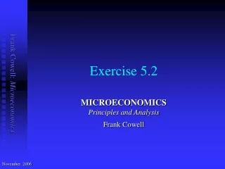
Exercise 5.2
Exercise 5.2. MICROECONOMICS Principles and Analysis Frank Cowell. November 2006. Ex 5.2(1): Question. purpose : construct a simple model of investment in the context of household supply method : combine answer to Ex 5.1 and a straightforward income-maximisation problem.

Exercise 5.2
E N D
Presentation Transcript
Exercise 5.2 MICROECONOMICS Principles and Analysis Frank Cowell November 2006
Ex 5.2(1): Question • purpose: construct a simple model of investment in the context of household supply • method: combine answer to Ex 5.1 and a straightforward income-maximisation problem
Ex 5.2(1): Find optimal investment • Net income is y = pR1+ R2 + bp[1 – e–z] – z • Maximise this where dy — = bpe–z– 1 = 0 dz • Solve this to get z = log (bp), which is positive if bp 1. • So optimal investment is z*(p,b) = max (log (bp), 0) • Note dependence on price p and on investment productivity b
Ex 5.2(2): Question method: • Use the result from part 1 • Work out the modified expression for income • Combine this with modified answer to Ex 5.1
Ex 5.2(2): Find supply of rice • Maximised income is y*(p,b)= pR1+ R2 + bp[1 – exp(–z*(p,b))] – z*(p,b) • Using the formula for optimal investment z* we find • if bp >1: y*(p,b)= pR1+ R2 + bp[1 – 1/bp] – log (bp)) = pR1+ R2 + bp– 1 – log (bp)) • otherwise y*(p,b)= pR1+ R2 • Total output of rice is now R1 + b[1 – exp(–z*(p,b))] • So, modifying answer to Ex 5.1, supply of rice is now y*(p,b)– k S*(p,b) = R1+ b[1 – exp(–z*(p,b))] – a ————— p • where a and k are parameters of the utility function • and y*(p,b) takes one of the two forms above • depends on whether or not p > 1/b
Ex 5.2(3): Question method: • Use the result from parts 1 and 2 • Differentiate with respect to p and b to get responses
Ex 5.2(3): Investment response • Optimal investment is z*(p,b) = max (log (bp), 0) • If p 1/b then, differentiating: z*(p,b) 1 ————= — > 0 p b z*(p,b)1 ————= — > 0 b p • Otherwise z* is constant at 0
Ex 5.2(3): Supply response (i) • If p 1/b maximised income is pR1+ R2 + bp– 1 – log (bp) • So supply of rice is R2– k – 1 – log (bp) S*(p,b) = [1–a ]R1+ ab– a ————————— p • Differentiating: S*(p,b)R2 –k – log (bp) ————= a——————— p p2 S*(p,b)1 – bp ————= a——— b bp • If R2 > k positive for small p • maybe negative for large p • non-positive
Ex 5.2(3): Supply response (ii) • If p < 1/b maximised income is pR1+ R2 • So supply of rice is R2– k S*(p,b) = R1– a ——— p • Differentiating: S*(p,b)R2 –k ————= a—— p p2 S*(p,b) ————= 0 b • If R2 > k positive for all p < 1/b
Ex 5.2: Points to remember • Make good use of answers to previous parts in each stage • When analysing optimal investment take care about the corner solution • Use the two cases (corner, interior solution) in modelling the agent’s response to price and productivity changes


