Understanding Stationarity in Time Series Analysis with Autoregressive and ARIMA Models
This guide explores the characteristics of stationary time series, specifically focusing on the Toeplitz covariance matrix, white noise properties, and the autoregressive moving average (ARIMA) models. It examines conditions for stationarity, forecasts using autoregressive order 1 models, and explores concepts like unit roots and mean reversion. Additionally, practical examples, including American Airlines stock volume data and the Nenana Ice Classic, are presented to demonstrate model fitting, residual checks, and the application of transfer functions in time series analysis.

Understanding Stationarity in Time Series Analysis with Autoregressive and ARIMA Models
E N D
Presentation Transcript
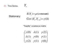
(1) Time Series Stationary: “Toeplitz” covariance matrix
(2) et: white noise—uncorrelated (0, σ2) [Wold representation]
(3)Example: if |r|<1 “Autoregressive order 1”Stationary? Yes if . Forecast L periods ahead: m + rL(Yn-m)
(5) Moving Average Order 1 Clearly stationary One step ahead forecast:
(7) Random Walk No Mean Revision Extends to higher order and mixed models
Note: EWMA = winner in CHANCE paper.
(9) Roots Yt-m = 1.2 (Yt-1-m) - .32(Yt-2-m)+et (1-1.2B+.32B2)(Yt-m )= et Division & partial fractions: (Yt-m ) = ( 2/(1-.8B) -1/(1-.4B) ) et convergent!
(1-1.2B+.32B2) roots: 1/.8, 1/.4 Yt-m = 1.2 (Yt-1-m) - .20(Yt-2-m)+et (1-1.2B+.2B2)(Yt-m ) = et (1-0.2B)(1-B) (1-0.2B)(Yt-Yt-1) = et “Unit root,” not stationary, no mean reversion. Studentized unit root tests (nonstandard) extend to higher order.
(10) Transfer function: Observe Intervention:
procarima data=AMERICAN; i var=volume crosscor=(WTC CRASH) noprint; e input = ( (1)/(1,2) WTC (1)/(1,2) CRASH) plot p=2 q=1; f lead=0 out=out1 id=date; where '01jan01'd < date < '01jan03'd; Standard Approx Parameter Estimate Error t Value Pr>|t| Lag Variable MU 1895175.1 241956.3 7.83 <.0001 0 volume MA1,1 0.80798 0.06487 12.45 <.0001 1 volume AR1,1 1.30707 0.08535 15.31 <.0001 1 volume AR1,2 -0.33545 0.07374 -4.55 <.0001 2 volume NUM1 15624717 831551.1 18.79 <.0001 0 WTC NUM1,1 -9564494.0 3086912.7 -3.10 0.0021 1 WTC DEN1,1 -0.21308 0.18425 -1.16 0.2481 1 WTC DEN1,2 0.38677 0.07282 5.31 <.0001 2 WTC NUM2 7534484.3 842654.2 8.94 <.0001 0 CRASH NUM1,1 4260018.6 2401054.1 1.77 0.0767 1 CRASH DEN1,1 0.79740 0.31164 2.56 0.0108 1 CRASH DEN1,2 0.04974 0.17505 0.28 0.7764 2 CRASH
Interpretation: Xt = WTC indicator 0 0 0 1 0 0 0 … Similarly for Xt = second crash indicator Error term is ARMA(2,1) Residual Checks Autocorrelation Check of Residuals To Chi- Pr > Lag Square DF ChiSq ---------Autocorrelations-------------- 6 11.07 3 0.0114 -0.002 -0.008 0.016 0.060 0.059 -0.121 12 13.69 9 0.1336 0.032 -0.019 -0.042 -0.030 -0.034 -0.002 18 20.49 15 0.1541 -0.082 -0.017 0.005 0.013 -0.074 0.023 24 37.27 21 0.0157 0.116 0.088 -0.087 -0.036 0.045 0.011 30 43.28 27 0.0245 -0.046 -0.016 0.059 -0.041 0.061 0.008 36 51.68 33 0.0203 0.069 0.013 -0.042 0.085 0.032 0.029 42 55.44 39 0.0425 -0.045 0.020 0.066 -0.002 -0.011 -0.002 48 56.92 45 0.1096 0.020 -0.011 -0.009 0.002 -0.005 0.046
Example 2: “Nenana Ice Classic” Start = 1917 pot is now $285,000
The ARIMA Procedure Conditional Least Squares Estimation Standard Approx Parameter Estimate Error t Value Pr > |t| Lag Variable MU 126.01962 0.59155 213.03 <.0001 0 break AR1,1 -0.21784 0.10929 -1.99 0.0494 6 break NUM1 -0.18686 0.04326 -4.32 <.0001 0 ramp Autocorrelation Check of Residuals To Chi- Pr > Lag Square DF ChiSq -------------Autocorrelations------------- 6 4.81 5 0.4399 -0.040 0.043 -0.064 0.054 -0.197 -0.034 12 14.37 11 0.2134 0.056 -0.089 -0.090 0.215 -0.023 -0.167 18 18.06 17 0.3850 -0.044 0.079 0.033 -0.060 0.129 -0.063 24 21.22 23 0.5679 -0.054 0.031 0.016 -0.123 -0.036 -0.075
** Using NLIN to estimate ramp start point **; proc nlin data=all; parms C=1960 a=126 b=-.2 ; X = (year-C)*(year>c); model break = a + b*X; run; NOTE: Convergence criterion met. Sum of Mean Approx Source DF Squares Square F Value Pr > F Model 2 403.5 201.7 6.35 0.0027 Error 85 2702.1 31.7894 Corrected Total 87 3105.6 Approx Approximate 95% Confidence Parameter Estimate Std Error Limits C 1967.6 10.7354 1946.2 1988.9 a 126.0 0.7895 124.4 127.6 b -0.1873 0.0868 -0.3599 -0.0147