Analyzing Climate Variability in South America: A Study with HadRM3P Regional Model
This study presents an analysis of climate variability in South America using the HadRM3P regional climate model, part of the CREAS program, which downscales climate data from the HadAM3P global model. Covering a period from 1961 to 1990, it evaluates the model's ability to reproduce precipitation and temperature patterns at a 50 km resolution. The results highlight the model's capability to simulate climatological features and assess its biases in predicting climate change scenarios, providing valuable insights for adaptation studies.

Analyzing Climate Variability in South America: A Study with HadRM3P Regional Model
E N D
Presentation Transcript
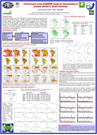
EXPERIMENTAL DESIGN Factors to consider Setup Research Components - Simulation length - Ensembles - Spin up - Choice of domain - Resolution - Output data - Surface configuration - 31 years (Jan/1960 to Dec/1990) - Three members - 1 year spin-up - South America - approximately 50Kmx50Km - standard diagnostics: daily - standard Model validation: - Assessing the consistency between the RCM and GCM - Assessing how well the RCM represents the present day climate Climate change scenario construction: - To generate high resolution climate change scenarios for use in climate impacts and adaptation studies. Brier Skill Score of the RCM for various rainfall indices in several regions. Anomaly correlation, considering the ensemble mean. Precipitation (top) and Temperature (below) Above area - 0.33 Below area - 0.40 Above area - 0.33 Below area - 0.45 OBSERVATION HadAM3P HadRM3P Above area - 0.57 Below area - 0.60 Precipitation (mm/dia) Above area - 0.60 Below area - 0.72 Above area - 0.50 Below area - 0.50 Above area - 0.78 Below area - 0.67 Temperature (ºC) Temperature (ºC) Hit rates versus false-alarm rates for seasonal area-averaged rainfall at the peak season for selected regions. Results are shown for the simulation of rainfall above (gray) and below (black). The area beneath the ROC curves is indicated also for above and below precipitation wind field at 850hPa wind field at 850hPa wind field at 200hPa wind field at 200hPa Regions of the SA Temperature Precipitation NAm NWP-E NNEB SAm SNEB SBr-U Nam = Amazonia (northern) Sam = Amazonia (southern) NNEB = Northeast Brazil (northern) SNEB = Northeast Brazil (southern) NWP-E = Northwest Peru-Equador SBr-U = Southern Brazil-Uruguay Temperature (ºC) Precipitation (mm/day) Performance of the HadRM3P model for downscaling of present climate in South American Lincoln Muniz Alves*, José A. Marengo* *Centro de Previsão de Tempo e Estudos Climáticos (CPTEC/INPE) 12630-000 Cachoeira Paulista, São Paulo, Brazil (Contact: lincoln@cptec.inpe.br) SKILL OF THE MODEL SIMULATION SCIENCE GOAL A regional program led by CPTEC/INPE is CREAS (Regional Climate Change Scenarios for South America). CREAS represents a collaboration between the UK-Met Hadley Centre Regional and various programs from the Brazilian government funded by GEF. In CREAS, the HadAM3P global model is used together with the HadRM3P regional model to downscale climate variability and change in South America at the resolution of 50 km. In this poster, we analyze simulations of climate variability for South America during the present (1961-1990), at the annual and seasonal levels. CONTROL CLIMATE SIMULATED BY THE RCM How far does the RCM diverge from its driving AGCM (HadAM3P)? How HadRM3P add value to the AGCM? OBSERVATION HadAM3P HadRM3P Precipitation (mm/dia) 1983 1985 • SUMMARY AND CONCLUSIONS • In general the HadRM3P is capalbe of simulating the mean climatological features over South America; • The HadRM3P resolves features on finer scales than the GCM. This is particularly clear for precipitation. • The model is found to represent quite accurately the primary features of observed circulation, temperature and precipitation patterns, including their seasonal cycle and the main modes of interannual variability. But, there are significant biases. • The model must be adequalety tuned in order to give reliabe for climate change, but there are a number of uncertainties and caveats associated with the RCM´s predictions of climate change over South America. Simulated precipitation, temperature and atmospheric circulation at 850 and 200 hPa for DFJ 1983 and 1985. HadAM3P (first column), HadRM3P (center), Observed (third column). REGIONAL CHARACTERISTICS AND TIME VARIABILITY Interannual variability of observed and modeled normalized rainfall departures during the peak of the rainy season. Tick black line represents the mean rainfall from the model ensemble. Thin blue lines represent each member of the ensemble. Tick red line shows the observed rainfall Table - Bias, standard deviation (STD), root mean square error (rmse) and correlation coefficient ()of annual cycle. Annual cycle of observed (CRU) and modeled rainfall and temperature in several regions of SA. Tick orange line shows observations. Thick black line represents the mean from the model ensemble. Others colors represent each member of the ensemble. Acknowledgements This poster is part of the a Master Degree Thesis of the first autor. We thank WMO and CPTEC for partially grants this conference. Thanks also to the UK-Met Office`s staffs for the valuable assistance. CREAS is funded by the UK FCO-GOF Program and the PROBIO-MMA-GEF project (Brazil)