Download

1 / 51
540 likes | 838 Vues
Tangent Lines and Arc Length Parametric Equations. Objective: Use the formulas required to find slopes, tangent lines, and arc lengths of parametric and polar curves. Parametric Equations.

E N D
Tangent Lines and Arc LengthParametric Equations Objective: Use the formulas required to find slopes, tangent lines, and arc lengths of parametric and polar curves.
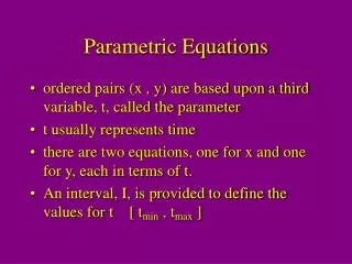
Parametric Equations • Suppose that a particle moves along a curve C in the xy-plane in such a way that its x- and y-coordinates, as functions of time, are and . We call these the parametric equations of motion for the particle and refer to C as the trajectory of the particle or the graph of the equations. The variable t is called the parameter for the equation.
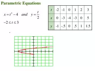
Example 1 • Sketch the trajectory over the time interval 0 < t < 10 of the particle whose parametric equations of motion are
Example 1 • Sketch the trajectory over the time interval 0 < t < 10 of the particle whose parametric equations of motion are • One way to sketch the trajectory is to choose a representative succession of times, plot the (x, y) coordinates of points on the trajectory at those times, and connect the points with a smooth curve.
Example 1 • Sketch the trajectory over the time interval 0 < t < 10 of the particle whose parametric equations of motion are • Observe that there is no t-axis; the values of t appear only as labels on the plotted points, and even these are usually omitted unless it is important to emphasize the location of the particle at specific times.
Example 1 • Although parametric equations commonly arise in problems of motion with time as the parameter, they arise in other contexts as well. Thus, unless the problem dictates that the parameter t in the equation represents time, it should be viewed simply as an independent variable that varies over some interval of real numbers. If no restrictions on the parameter are stated explicitly or implied by the equations, then it is understood that it varies from
Example 2 • Find the graph of the parametric equations
Example 2 • Find the graph of the parametric equations • One way to find the graph is to eliminate the parameter t by noting that Thus the graph is contained in the unit circle. Geometrically, the parameter t can be interpreted as the angle swept out by the radial line from the origin to the point (x, y) = (cost, sint) on the unit circle. As t increases from 0 to 2p, the point traces the circle counterclockwise.
Orientation • The direction in which the graph of a pair of parametric equations is traced as the parameter increases is called the direction of increasing power or sometimes the orientation imposed on the curve by the equations. Thus, we make a distinction between a curve, which is a set of points, and a parametric curve, which is a curve with an orientation imposed on it by a set of parametric equations.
Orientation • For example, we saw in example 2 that the circle represented parametrically is traced counterclockwise as t increases and hence has counterclockwise orientation. • To obtain parametric equations for the unit circle with clockwise orientation, we can replace t by –t.
Example 3 • Graph the parametric curve by eliminating the parameter and indicate the orientation on the graph.
Example 3 • Graph the parametric curve by eliminating the parameter and indicate the orientation on the graph. • To eliminate the parameter we will solve the first equation for t as a function of x, and then substitute this expression for t into the second equation.
Example 3 • Graph the parametric curve by eliminating the parameter and indicate the orientation on the graph. • The graph is a line of slope 3 and y-intercept 2. To find the orientation we must look at the original equations; the direction of increasing t can be deduced by observing that x increases as t increases or that y increases as t increases.
Tangent Lines to Parametric Curves • We will be concerned with curves that are given by parametric equations x = f(t) and y = g(t) in which f(t) and g(t) have continuous first derivatives with respect to t. If can be proved that if dx/dt is not zero, then y is a differentiable function of x, in which case the chain rule implies that • This formula makes it possible to find dy/dx directly from the parametric equations without eliminating the parameter.
Example 1 • Find the slope of the tangent line to the unit circle at the point where
Example 1 • Find the slope of the tangent line to the unit circle at the point where • The slope at a general point on the circle is • The slope at is
Tangent Lines • It follows from the formula that the tangent line to a parametric curve will be horizontal at those points where dy/dt = 0 and dx/dt does not (0/#).
Tangent Lines • It follows from the formula that the tangent line to a parametric curve will be horizontal at those points where dy/dt = 0 and dx/dt does not (0/#). • Two different situations occur when dx/dt = 0. At points where dx/dt =0 and dy/dt does not (#/0), the tangent line has infinite slope and a vertical tangent line at such points.
Tangent Lines • It follows from the formula that the tangent line to a parametric curve will be horizontal at those points where dy/dt = 0 and dx/dt does not (0/#). • Two different situations occur when dx/dt = 0. At points where dx/dt =0 and dy/dt does not (#/0), the tangent line has infinite slope and a vertical tangent line at such points. • When dx/dt and dy/dt =0, we call such point singular points. No general statement can be made about singular points; they must be analyzed case by case.
Example 2 • In a disastrous first flight, an experimental paper airplane follows the trajectory but crashes into a wall at time t = 10. (a) At what times was the airplane flying horizontally? (b) At what times was it flying vertically?
Example 2 • In a disastrous first flight, an experimental paper airplane follows the trajectory but crashes into a wall at time t = 10. (a) At what times was it flying horizontally? (a) The airplane was flying horizontally at those times when dy/dt = 0 and dx/dt does not.
Example 2 • In a disastrous first flight, an experimental paper airplane follows the trajectory but crashes into a wall at time t = 10. (b) At what times was it flying vertically? (b) The airplane was flying vertically at those times when dx/dt = 0 and dy/dt does not.
Example 3 • The curve represented by the parametric equations is called a semicubical parabola. The parameter t can be eliminated by cubing x and squaring y, from which it follows the y2 = x3. The graph of this equation consists of two branches; an upper branch obtained by graphing y = x3/2 and a lower branch obtained by graphing y = -x3/2.
Example 4 • Without eliminating the parameter, find and at (1, 1) and (1, -1) on the simicubical parabola given in example 3.
Example 4 • Without eliminating the parameter, find and at (1, 1) and (1, -1) on the simicubical parabola given in example 3.
Example 4 • Without eliminating the parameter, find and at (1, 1) and (1, -1) on the simicubical parabola given in example 3. • Since the point (1, 1) on the curves corresponds to t = 1 in the parametric equations, it follows that
Example 4 • Without eliminating the parameter, find and at (1, 1) and (1, -1) on the simicubical parabola given in example 3. • Since the point (1, -1) on the curves corresponds to t = -1 in the parametric equations, it follows that
Tangent Lines to Polar Curves • Our next objective is to find a method for obtaining slopes of tangent lines to polar curves of the form r = f(q) in which r is a differentiable function of q. A curve of this form can be expressed parametrically in terms of the parameter q by substituting f(q) for r in the equation x = rcosq and y = rsinq. This yields
Tangent Lines to Polar Curves • From this we obtain
Tangent Lines to Polar Curves • Thus, if and are continuous and if then y is a differentiable function of x, and with q in place of t yields
Example 5 • Find the slope of the tangent line to the circle r =4cosq at the point where .
Example 5 • Find the slope of the tangent line to the circle r =4cosq at the point where . • Substituting into the formula gives
Example 5 • Find the slope of the tangent line to the circle r =4cosq at the point where . • Substituting into the formula gives
Example 6 • Find the points on the cardioid r = 1 – cosq at which there is a horizontal tangent line, a vertical tangent line, or a singular point.
Example 6 • Find the points on the cardioid r = 1 – cosq at which there is a horizontal tangent line, a vertical tangent line, or a singular point. • This is easiest if we express the cardioid parametrically by substituting r = 1 – cosq into the conversion formulas x = rcosq and y = rsinq. This yields
Example 6 • Find the points on the cardioid r = 1 – cosq at which there is a horizontal tangent line, a vertical tangent line, or a singular point. • A horizontal tangent occurs when
Example 6 • Find the points on the cardioid r = 1 – cosq at which there is a horizontal tangent line, a vertical tangent line, or a singular point. • A vertical tangent occurs when
Example 6 • Find the points on the cardioid r = 1 – cosq at which there is a horizontal tangent line, a vertical tangent line, or a singular point. • A singular point occurs when
Tangent Lines to Polar Curves at the Origin • The following theorem could prove useful.
Tangent Lines to Polar Curves at the Origin • The following theorem could prove useful. • This theorem tells us that equations of the tangent lines at the origin to the curve r = f(q) can be obtained by solving the equation f(q) = 0. It is important to keep in mind that r = f(q) may be zero for more than one value of q, so there may be more than one tangent line at the origin.
Example 7 • The three-petal rose r = sin3q has three tangent lines at the origin, which can be found by solving the equation sin3q = 0. The solutions are
Arc Length of a Polar Curve • A formula for the arc length of a polar curve r = f(q) can be derived by expressing the curve in parametric form and applying the formula for the are length of a parametric curve.
Arc Length of a Polar Curve • A formula for the arc length of a polar curve r = f(q) can be derived by expressing the curve in parametric form and applying the formula for the are length of a parametric curve.
Example 8 • Find the arc length of the spiral r = eq between q = 0 and q = p.
Example 8 • Find the arc length of the spiral r = eq between q = 0 and q = p.
Example 9 • Find the total arc length of the cardioid r = 1 + cosq.
Example 9 • Find the total arc length of the cardioid r = 1 + cosq.
Example 9 • Find the total arc length of the cardioid r = 1 + cosq.
Example 9 • Find the total arc length of the cardioid r = 1 + cosq.
Other Important Ideas • Here are some formulas that you will need to know for the AP Exam. These are not in the book.