Download

1 / 43
430 likes | 447 Vues
Learn to minimize communication in linear algebra for faster algorithms with optimal message-passing techniques. Discover the key to achieving exponential improvements in running time and bandwidth utilization.

E N D
Avoiding Communicationin Linear Algebra Jim Demmel UC Berkeley bebop.cs.berkeley.edu
Motivation • Running time of an algorithm is sum of 3 terms: • # flops * time_per_flop • # words moved / bandwidth • # messages * latency communication
Motivation • Running time of an algorithm is sum of 3 terms: • # flops * time_per_flop • # words moved / bandwidth • # messages * latency • Exponentially growing gaps between • Time_per_flop << 1/Network BW << Network Latency • Improving 59%/year vs 26%/year vs 15%/year • Time_per_flop << 1/Memory BW << Memory Latency • Improving 59%/year vs 23%/year vs 5.5%/year communication
Motivation • Running time of an algorithm is sum of 3 terms: • # flops * time_per_flop • # words moved / bandwidth • # messages * latency • Exponentially growing gaps between • Time_per_flop << 1/Network BW << Network Latency • Improving 59%/year vs 26%/year vs 15%/year • Time_per_flop << 1/Memory BW << Memory Latency • Improving 59%/year vs 23%/year vs 5.5%/year • Goal : reorganize linear algebra to avoid communication • Notjust hiding communication (speedup 2x ) • Arbitrary speedups possible communication
Outline • Motivation • Avoiding Communication in Dense Linear Algebra • Avoiding Communication in Sparse Linear Algebra
Outline • Motivation • Avoiding Communication in Dense Linear Algebra • Avoiding Communication in Sparse Linear Algebra • A poem in memory of Gene Golub (separate file)
Collaborators (so far) • UC Berkeley • Kathy Yelick, Ming Gu • Mark Hoemmen, MarghoobMohiyuddin, KaushikDatta, George Petropoulos, Sam Williams, BeBOp group • Lenny Oliker, John Shalf • CU Denver • JulienLangou • INRIA • Laura Grigori, Hua Xiang • Much related work • Complete references in technical reports
Why all our problems are solved for dense linear algebra– in theory • (Talk by IoanaDumitriu on Monday) • Thm (D., Dumitriu, Holtz, Kleinberg) (Numer.Math. 2007) • Given any matmul running in O(n) ops for some >2, it can be made stable and still run in O(n+) ops, for any >0. • Current record: 2.38 • Thm (D., Dumitriu, Holtz) (Numer. Math. 2008) • Given any stable matmul running in O(n+) ops, it is possible to do backward stable dense linear algebra in O(n+) ops: • GEPP, QR • rank revealing QR (randomized) • (Generalized) Schur decomposition, SVD (randomized) • Also reduces communication to O(n+) • But constants?
Summary (1) – Avoiding Communication in Dense Linear Algebra • QR or LU decomposition of m x n matrix, m >> n • Parallel implementation • Conventional: O( n log p ) messages • “New”: O( log p ) messages - optimal • Serial implementation with fast memory of size F • Conventional: O( mn/F ) moves of data from slow to fast memory • mn/F = how many times larger matrix is than fast memory • “New”: O(1) moves of data - optimal • Lots of speed up possible (measured and modeled) • Price: some redundant computation, stability? • Extends to square case, with optimality results • Extends to other architectures (egmulticore) • (Talk by JulienLangou Monday, on QR)
R00 R10 R20 R30 W0 W1 W2 W3 R01 W = R02 R11 Minimizing Comm. in Parallel QR • QR decomposition of m x n matrix W, m >> n • TSQR = “Tall Skinny QR” • P processors, block row layout • Usual Parallel Algorithm • Compute Householder vector for each column • Number of messages n log P • Communication Avoiding Algorithm • Reduction operation, with QR as operator • Number of messages log P
TSQR in more detail Q is represented implicitly as a product (tree of factors)
Minimizing Communication in TSQR R00 R10 R20 R30 W0 W1 W2 W3 R01 Parallel: W = R02 R11 R00 W0 W1 W2 W3 Sequential: R01 W = R02 R03 R00 R01 W0 W1 W2 W3 R01 Dual Core: W = R02 R11 R03 R11 Multicore / Multisocket / Multirack / Multisite / Out-of-core: ? Choose reduction tree dynamically
Performance of TSQR vsSca/LAPACK • Parallel • Pentium III cluster, Dolphin Interconnect, MPICH • Up to 6.7x speedup (16 procs, 100K x 200) • BlueGene/L • Up to 4x speedup (32 procs, 1M x 50) • Both use Elmroth-Gustavson locally – enabled by TSQR • Sequential • OOC on PowerPC laptop • As little as 2x slowdown vs (predicted) infinite DRAM • See UC Berkeley EECS Tech Report 2008-74
QR for General Matrices • CAQR – Communication Avoiding QR for general A • Use TSQR for panel factorizations • Apply to rest of matrix • Cost of CAQR vsScaLAPACK’sPDGEQRF • n x n matrix on P1/2 x P1/2 processor grid, block size b • Flops: (4/3)n3/P + (3/4)n2b log P/P1/2 vs(4/3)n3/P • Bandwidth: (3/4)n2 log P/P1/2vssame • Latency: 2.5 n log P / bvs1.5 n log P • Close to optimal (modulo log P factors) • Assume: O(n2/P) memory/processor, O(n3) algorithm, • Choose b near n / P1/2 (its upper bound) • Bandwidth lower bound: (n2 /P1/2) – just log(P) smaller • Latency lower bound: (P1/2) – just polylog(P) smaller • Extension of Irony/Toledo/Tishkin (2004) • Implementation – Julien’s summer project
Modeled Speedups of CAQR vs ScaLAPACK Petascale up to 22.9x IBM Power 5 up to 9.7x “Grid” up to 11x Petascale machine with 8192 procs, each at 500 GFlops/s, a bandwidth of 4 GB/s.
TSLU: LU factorization of a tall skinny matrix First try the obvious generalization of TSQR:
Growth factor for TSLU based factorization • Unstable for large P and large matrices. • When P = # rows, TSLU is equivalent to parallel pivoting. Courtesy of H. Xiang
Making TSLU Stable • At each node in tree, TSLU selects b pivot rows from 2b candidates from its 2 child nodes • At each node, do LU on 2b original rows selected by child nodes, not U factors from child nodes • When TSLU done, permute b selected rows to top of original matrix, redo b steps of LU without pivoting • CALU – Communication Avoiding LU for general A • Use TSLU for panel factorizations • Apply to rest of matrix • Cost: redundant panel factorizations • Benefit: • Stable in practice, but not same pivot choice as GEPP • b times fewer messages overall - faster
Growth factor for better CALU approach Like threshold pivoting with worst case threshold = .33 , so |L| <= 3 Testing shows about same residual as GEPP
Performance vs ScaLAPACK • TSLU • IBM Power 5 • Up to 4.37x faster (16 procs, 1M x 150) • Cray XT4 • Up to 5.52x faster (8 procs, 1M x 150) • CALU • IBM Power 5 • Up to 2.29x faster (64 procs, 1000 x 1000) • Cray XT4 • Up to 1.81x faster (64 procs, 1000 x 1000) • Optimality analysis analogous to QR • See INRIA Tech Report 6523 (2008)
Speedup prediction for a Petascale machine - up to 81x faster P = 8192 Petascale machine with 8192 procs, each at 500 GFlops/s, a bandwidth of 4 GB/s.
Summary (2) – Avoiding Communication in Sparse Linear Algebra • Take k steps of Krylov subspace method • GMRES, CG, Lanczos, Arnoldi • Assume matrix “well-partitioned,” with modest surface-to-volume ratio • Parallel implementation • Conventional: O(k log p) messages • “New”: O(log p) messages - optimal • Serial implementation • Conventional: O(k) moves of data from slow to fast memory • “New”: O(1) moves of data – optimal • Can incorporate some preconditioners • Hierarchical, semiseparable matrices … • Lots of speed up possible (modeled and measured) • Price: some redundant computation
Locally Dependent Entries for [x,Ax], A tridiagonal, 2 processors A8x A7x A6x A5x A4x A3x A2x Ax x Proc 1 Proc 2 Can be computed without communication
Locally Dependent Entries for [x,Ax,A2x], A tridiagonal, 2 processors A8x A7x A6x A5x A4x A3x A2x Ax x Proc 1 Proc 2 Can be computed without communication
Locally Dependent Entries for [x,Ax,…,A3x], A tridiagonal, 2 processors A8x A7x A6x A5x A4x A3x A2x Ax x Proc 1 Proc 2 Can be computed without communication
Locally Dependent Entries for [x,Ax,…,A4x], A tridiagonal, 2 processors A8x A7x A6x A5x A4x A3x A2x Ax x Proc 1 Proc 2 Can be computed without communication
Locally Dependent Entries for [x,Ax,…,A8x], A tridiagonal, 2 processors A8x A7x A6x A5x A4x A3x A2x Ax x Proc 1 Proc 2 Can be computed without communication k=8 fold reuse of A
A8x A7x A6x A5x A4x A3x A2x Ax x Remotely Dependent Entries for [x,Ax,…,A8x], A tridiagonal, 2 processors Proc 1 Proc 2 One message to get data needed to compute remotely dependent entries, not k=8 Minimizes number of messages = latency cost Price: redundant work “surface/volume ratio”
A8x A7x A6x A5x A4x A3x A2x Ax x Fewer Remotely Dependent Entries for [x,Ax,…,A8x], A tridiagonal, 2 processors Proc 1 Proc 2 Reduce redundant work by half
Remotely Dependent Entries for [x,Ax,A2x,A3x], A irregular, multiple processors
Sequential [x,Ax,…,A4x], with memory hierarchy v One read of matrix from slow memory, not k=4 Minimizes words moved = bandwidth cost No redundant work
Performance Results • Measured • Sequential/OOC speedup up to 3x • Modeled • Sequential/multicore speedup up to 2.5x • Parallel/Petascale speedup up to 6.9x • Parallel/Grid speedup up to 22x • See bebop.cs.berkeley.edu/#pubs
Optimizing Communication Complexity of Sparse Solvers • Example: GMRES for Ax=b on “2D Mesh” • x lives on n-by-n mesh • Partitioned on p½ -by- p½ grid • A has “5 point stencil” (Laplacian) • (Ax)(i,j) = linear_combination(x(i,j), x(i,j±1), x(i±1,j)) • Ex: 18-by-18 mesh on 3-by-3 grid
Minimizing Communication of GMRES • What is the cost = (#flops, #words, #mess) of k steps of standard GMRES? GMRES, ver.1: for i=1 to k w = A * v(i-1) MGS(w, v(0),…,v(i-1)) update v(i), H endfor solve LSQ problem with H n/p½ n/p½ • Cost(A * v) = k * (9n2 /p, 4n / p½ , 4 ) • Cost(MGS) = k2/2 * ( 4n2 /p , log p , log p ) • Total cost ~ Cost( A * v ) + Cost (MGS) • Can we reduce the latency?
GMRES, ver. 2: W = [ v, Av, A2v, … , Akv ] [Q,R] = MGS(W) Build H from R, solve LSQ problem k = 3 • Cost(W) =( ~ same, ~ same, 8 ) • Latency cost independent of k – optimal • Cost (MGS) unchanged • Can we reduce the latency more? Minimizing Communication of GMRES • Cost(GMRES, ver.1) = Cost(A*v) + Cost(MGS) = ( 9kn2 /p, 4kn / p½ , 4k ) + ( 2k2n2 /p , k2 log p / 2 , k2 log p / 2 ) • How much latency cost from A*v can you avoid? Almost all
GMRES, ver. 3: W = [ v, Av, A2v, … , Akv ] [Q,R] = TSQR(W) … “Tall Skinny QR” Build H from R, solve LSQ problem R1 R2 R3 R4 W1 W2 W3 W4 R12 W = R1234 R34 • Cost(TSQR) =( ~ same, ~ same, log p ) • Latency cost independent of s - optimal Minimizing Communication of GMRES • Cost(GMRES, ver. 2) = Cost(W) + Cost(MGS) = ( 9kn2 /p, 4kn / p½ , 8 ) + ( 2k2n2 /p , k2 log p / 2 , k2 log p / 2 ) • How much latency cost from MGS can you avoid? Almost all
R1 R2 R3 R4 W1 W2 W3 W4 R12 W = R1234 R34 • Cost(TSQR) =( ~ same, ~ same, log p ) • Oops Minimizing Communication of GMRES • Cost(GMRES, ver. 2) = Cost(W) + Cost(MGS) = ( 9kn2 /p, 4kn / p½ , 8 ) + ( 2k2n2 /p , k2 log p / 2 , k2 log p / 2 ) • How much latency cost from MGS can you avoid? Almost all GMRES, ver. 3: W = [ v, Av, A2v, … , Akv ] [Q,R] = TSQR(W) … “Tall Skinny QR” Build H from R, solve LSQ problem
R1 R2 R3 R4 W1 W2 W3 W4 R12 W = R1234 R34 • Cost(TSQR) =( ~ same, ~ same, log p ) • Oops – W from power method, precision lost! Minimizing Communication of GMRES • Cost(GMRES, ver. 2) = Cost(W) + Cost(MGS) = ( 9kn2 /p, 4kn / p½ , 8 ) + ( 2k2n2 /p , k2 log p / 2 , k2 log p / 2 ) • How much latency cost from MGS can you avoid? Almost all GMRES, ver. 3: W = [ v, Av, A2v, … , Akv ] [Q,R] = TSQR(W) … “Tall Skinny QR” Build H from R, solve LSQ problem
Minimizing Communication of GMRES • Cost(GMRES, ver. 3) = Cost(W) + Cost(TSQR) = ( 9kn2 /p, 4kn / p½ , 8 ) + ( 2k2n2 /p , k2 log p / 2 , log p ) • Latency cost independent of k, just log p – optimal • Oops – W from power method, so precision lost – What to do? • Use a different polynomial basis • Not Monomial basis W = [v, Av, A2v, …], instead … • Newton Basis WN = [v, (A – θ1 I)v , (A – θ2 I)(A – θ1 I)v, …] or • Chebyshev Basis WC = [v, T1(v), T2(v), …]
Summary and Conclusions (1/2) • Possible to minimize communication complexity of much dense and sparse linear algebra • Practical speedups • Approaching theoretical lower bounds • Optimal asymptotic complexity algorithms for dense linear algebra – also lower communication • Hardware trends mean the time has come to do this • Lots of prior work (see pubs) – and some new
Summary and Conclusions (2/2) • Many open problems • Automatic tuning - build and optimize complicated data structures, communication patterns, code automatically: bebop.cs.berkeley.edu • Extend optimality proofs to general architectures • Dense eigenvalue problems – SBR or spectral D&C? • Sparse direct solvers – CALU or SuperLU? • Which preconditioners work? • Why stop at linear algebra?