Download
1 / 15
220 likes | 892 Vues
Lec 28, Ch.20, pp.955-973: Flexible pavement design, ESAL (Objectives). Know the structural components of a flexible pavement Learn the types of soil stabilization methods (from reading) Learn the general principles of flexible pavement design Know how to estimate equivalent single axle load.

E N D
Lec 28, Ch.20, pp.955-973: Flexible pavement design, ESAL (Objectives) • Know the structural components of a flexible pavement • Learn the types of soil stabilization methods (from reading) • Learn the general principles of flexible pavement design • Know how to estimate equivalent single axle load
What we discuss in class today… • Structural components of a flexible pavement • Wheel load pressure and pavement structure • Converting the repetition of wheel loads to the values that can be used for pavement design
Pavement types Flexible Pavement Rigid Pavement (Portland Cement) AC surface (3 to 6 in) PC surface (6 to 12 in) Granular base (Base course) Subbase Base course Subgrade Subgrade
Structural components of a flexible pavement Asphalt concrete surface: Mixture of mineral aggregates and asphaltic materials. 3” to 6” depending on the expected traffic on the pavement. Granular base (Base course): Usually granular materials such as crushed stone, crushed or uncrushed slag, crushed or uncrushed gravel, and sand. Subbase: Located immediately above the subgrade. Material of a superior quality than the subgrade. If necessary, it may be ‘stabilized.” Subgrade: Usually the natural material located along the horizontal alignment of the pavement and serves as the foundation of the pavement structure. May be a layer of selected borrowed materials, well compacted. Remember once loosened, soil must be compacted to reduce voids.
Load distribution through the pavement structure (covered by CE563) • Typical assumptions: • Multilayered elastic system • Subbase, base course, AC surface is infinite in the horizontal direction • Subgrade is infinite in the vertical and horizontal direction Higher strength materials needed • Contain both the horizontal and vertical strains below the set values that will cause excessive cracking • These criteria are considered in terms of repeated load applications because the accumulated repetitions of traffic loads are of significant importance to the development of cracks and permanent deformation of the pavement.
Estimating accumulated wheel load repetitions Traffic Characteristics: The traffic characteristics are determined in terms of the number of repetitions of an 18,000-lb (80 kilo-newtons (kN)) single-axle load applied to the pavement on two sets of dual tires. Equivalent single-axle load (ESAL) • Tire contact area (each 4.51in. (11 cm) radius) and 13.57 (33 cm) in apart • Contact pressure of 70 lb/in2 Premise: “the effect of any load on the performance of a pavement can be represented in terms of the number of single applications of an 18,000-lb single axle. 4 tires x x 4.512 = 255.601 in2, Total single-axle load = 255.601 x 70 lb/in2 = 17,892 approximately 18,000 lbs.
Load equivalency factors (Table 20.3): Use this if you know axle loads Obviously the traffic mix (cars, buses, SU trucks, semis, etc.) must be known because their gross axle loads are different. Vehicle classification counts are needed. Also needed is axle load data – the reason for having truck weighing stations on major highways.
How to estimate the traffic mix if field data are not available (In this case axle loads data must be available). Table 20.4 can help you estimate break-down of truck types in percentages. % %
How to estimate ESAL if axle loads are not known The equivalent 18,000-lb loads can also be determined from the vehicle type, if the axle load is unknown, by using a truck factor for that vehicle type. The truck factor is defined as the number of 18,000-lb single-load applications caused by a single passage of a vehicle. Table 20.5 gives truck factors, that is, they were computed based on previous research data. Remember this formula as the definition of the truck factor. You may not actually compute it unless you are determining typical truck factors for your study area. Problem 20-4 let you use this formula.
Distribution of truck factors for different classes of highways and vehicles Example: For rural interstates, one single truck is considered to have 0.52 ESAL. Count the total number of trucks and multiply it by 0.52 to find total ESAL for that section.
Determining the accumulated ESAL Must know: Design period, traffic growth rate, and design lane factor. Usually a 20-year design period is used. Traffic growth rates can be obtained from the planning division of the State DOT. Design lane factor: Pavement design is done for the highest loading case (design lane). Typically the outer lane is subject to the highest loading. Growth factor for a given growth rate j and design period t
Determining accumulated ESAL when axle loads are used • ESALi = equivalent accumulated 18,000-lb (80kN) single-axle load for the axle category i • fd = design lane factor • Gjt = growth factor for a given growth rate j and design period t • AADTi = first year annual average daily traffic for axle category i • Ni = number of axles on each vehicle in axle category i • FEi = load equivalency factor for axle category i Note that AADT used here is the total for both directions.
Determining accumulated ESAL when truck factors are used The accumulated ESAL for all categories of axle loads is: • ESALi = equivalent accumulated 18,000-lb axle load for truck category i • fd = design lane factor • Gjt = growth factor for a given growth rate j and design period t • AADTi = first year annual average daily traffic for truck category i • fi = truck factor for vehicles in truck category i • ESAL = equivalent accumulated 18,000-lb axle loads for all vehicles • n = number of truck categories
Example 20-1: Using load equivalency factors • Given: • 8-lane divided highway with AADT = 12,000 in each direction • PC (1,000lb/axle) = 50%, 2-axle SU (6,000lb/axle) = 33%, 3-axle SU (10,000lb/axle) = 17% • 4% annual growth in traffic • Design period 20 yrs • Values extracted from tables: • Gjt = 29.78 (Table 20.6) • fd = 40% = 0.40 (Table 20.7, 6 or more lanes) • Load equivalency factor (Table 20.3) Passenger Car Fei = 0.00002 (negligible) 2-axle Single Unit Fei = 0.01043 3-axle Single Unit Fei = 0.0877 2-axle SU trucks = 0.40 x 29.78 x 12000 x 0.33 x 365 x 2 x 0.01043 = 0.3592 x 10⁶ 3-axle SU trucks = 0.40 x 29.78 x 12000 x 0.17 x 365 x 3 x 0.0877 = 2.3336 x 10⁶ Total ESAL = (0.3592 + 2.3336) x 106 = 2.6928 x 10⁶
Example 20-2 • Given: • 2-lane major rural collector • AADT = 3000 (both directions) • Traffic growth rate = 5% • Design period = 20 yrs • Passenger Car 60% • SU trucks: 2-axle 4-tire 18%, 2-axle 6-tire 8%, 3-axle or more = 4% • Semi & combinations: 4-axle or less = 4% See Table 20-2 for the computations. fd = 0.5 in this case (even distribution in both directions) Gjt = 33.06 (Table 20.6)