Download
1 / 30
310 likes | 447 Vues
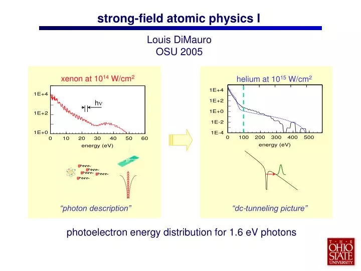
strong-field atomic physics I. xenon at 10 14 W/cm 2. helium at 10 15 W/cm 2. h n. “photon description”. “dc-tunneling picture”. photoelectron energy distribution for 1.6 eV photons. Louis DiMauro OSU 2005. strong-field atomic physics I. . [ o int (t ) ]( t ) iħ ( t ).

E N D
strong-field atomic physics I xenon at 1014 W/cm2 helium at 1015 W/cm2 hn “photon description” “dc-tunneling picture” photoelectron energy distribution for 1.6 eV photons Louis DiMauro OSU 2005
strong-field atomic physics I [o int(t)](t) iħ(t) time-dependent Schrődinger equation • understand the limit where Hint Ho • probe on a time-scale where t < to • guide dynamics by tailoring Hint(t) Louis DiMauro OSU 2005
photoelectric effect Einstein (1905) Ee 0 h ip electron energy Ee= h - ip transition probability: P = Fwhere cm2, F /cm2 s, s consider cw-light: = (1A)2 = 10-16 cm2for P 1: F ~ 1016 /cm2 sor intensity I ~ 10-3 W/cm2 100 fs (10-13 s) light pulse:for P 1: F ~ 1029 /cm2 sor intensity I ~ 1010 W/cm2
multi-photon photoelectric effect n-photon case (h ip) Ee Ee 0 h b 0 ip ip a h electron energy Ee=2h - ip electron energy Ee=nh - ip h ~ 0 transition probability: P = nFn where n cm2n sn-1 2-photon case (h ip) transition probability: P = aF bF or P = 2F2 where 2 a b = cm4 s
dc-tunnel ionization coulomb -1/x dc field -xE stark -1/x - xE DC field xE Stark -1/x + xE - + - + + - + - V + = = x x x x x Tunnel Rate 1/E eE
ac-tunnel ionization electron current E-field • electrons are emitted as burst every ½-cycle.
Keldysh (1964) theory of ionization optical frequency tunneling frequency << 1 tunneling low frequency and/or high intensity >> 1 multiphoton high frequency and/or low intensity “dc-tunneling picture” “photon description”
hydrogen atom r=510-9 cm Coulomb Law E= q/r2 ~ 5109 V/cm 1au + - What laser intensity gives an equivalent field strength?
above-threshold ionization (ATI) à la Agostini S=0 1.06 m, 4 1013 W/cm2 0.53 m, 8 1012 W/cm2 S=1 Xe: Ip =12.1 eV Ee = Nh - Ip 0.53 m, N=6, EN=1.9 eV 1.06 m, N=11, EN=0.77 eV ATI: N+S = (N+S)h - Ip 0.53 m, S=1, E7=4.2 eV
motion of the free electron • ponderomotive or quiver energy:Upl2 /4 • displacement:a l2 E • For 800 nm (red) laser at 1015 W/cm2Up= 60 eVa ~ 50 au (25 A) think in ponderomotive units !!!
ATI & ponderomotive threshold shift h +Up(I) ionization energy ionization energy perturbation theory f()=2n P2n(cos) Xe Xe Xe+ Xe+ N+S() = (N+S)h - Ip – Up() intensity-dependent energy • xenon • long pulse, 30 ps • 1 m , 30 TW/cm2
ponderomotive acceleration y x • electrons are repelled from regions of high intensity. • long pulse (adiabatic)quiver E translational N+S(r,) = (N+S)h - Ip–Up(r,) + Up(r,) intensity-independent energy
short pulse “resonant” ATI • Xenon, 100 fs, 800 nm, 70 TW/cm2 Freeman et al. PRL 59, 1092 (1987) for short pulse the ponderomotive gradient is negligible.
role of resonance electron energy electron energy electron energy electron energy electron energy E E E E • Experiment is a spatial and temporal average of intensity I(r,t). 0 0 0 0 0 E I
the simpleman’s picture of ionization o Field amplitude 2 Time • quasi-classical description: • Gallagher, PRL 61, 2304 (1988) • Van Linden van den Heuvell & Muller, in Multiphoton Processes (1988) • Corkum, Burnett & Brunel, PRL 62, 1259 (1989) electric fieldE = Eo sint velocityv(t) = Eo/[cost - coso] + vo quiver drift for tunneling, vo=0
predictions of the simpleman • in the experiment, we detect the drift energy not quiver !! T = mv2/2 = 2Up cos2 o V x V Tunnel Rate 1/E eE • Maximum drift energy = 2Up. x v(t) = Eo/[cost - coso] QuiverDrift
simpleman comparison to experiment 1 xenon 30 TW/cm2 Up = 3 eV bad news! helium 1 PW/cm2 Up = 50 eV good news! remember Up !!!
simpleman comparison to experiment 2 Agostini, Muller et al. Simpleman sideband estimate: v(t) = Eo/[cost - coso] + vo with vo kinetic energy 1s22s22p63s23p6 1s22s22p53s23p6 L-shell ionization broadening: e(200 eV) + dressing experiment: To = 200 eV, Up = 20 meV T = 6 sidebands good simpleman!
moving beyond the simpleman quantum model: TDSE-SAE K. Schafer et al. PRL 70, 1599 (1993) ~ 10-4–5 helium, 0.8 m, 1 PW/cm2 ideal case 10 Hz & 100 channel experiment: 100 e/shot or 1 e/ch*s, 105 range 28 hrs!
1 au field adequate for atomic physics? • n-photon ionization perturbation theory: P = n Fn • saturation (depletion): P Fs = (n )-1/n • helium (24 eV, 16-photons): • Fs = 1033 p/s*cm2 or Es ~ 0.1 au • over-the-barrier ionization • V(x) = -Ze2/x – eEox • solve for Eo: • Eo = Ip2/4q3Z • helium: Eo = 0.2 au answer: 1 au field is adequate for neutral atomic ionization!
for high sensitivity measurements baseline: 1 au field strength (3.5 1016 W/cm2) pulse: 100 fs duration & 4 m beam waist 1 mJ pulse energy typical laser produces a few Watts average power 103 pulses per second • kilohertz regenerative amplification (late 1980s): • Mourou, Bado, Bouvier (Rochester) • Saeed, Kim, DiMauro (BNL) • Fayer (Stanford) • … • seminal work (LLNL): • Lowdermilk & Murray, J App. Phys. 51, 2436 (1980).
for kilohertz regenerative amplification • cw or quasi-cw pumping • factors: absorption spectrum, lifetime, thermal coefficients, … • material properties • damage, saturation fluence, … • YLF, YAG, glass: millisecond lifetimes, broad absorption • poor thermal properties, narrow emission • Ti:sapphire: microsecond lifetimes, narrow absorption • good thermal properties, broad emission • advantages of regenerative amplification: • high amplification 106-8 • excellent spatial mode • good stability 1-3% rms
kHz regenerative amp circa MDCCCCLXXXVIII AD PD1 dump HR HR Q-switch & trap Pockels cell YLF head coupling polarizers out PD1 PD1
for amplifying short pulse ultra-fast laser oscillator 1000x stretcher amplifier media 1000x compressor positive GVD negative GVD Chirped Pulse Amplification (CPA) * G. Mourou and Strickland (1985) • extract maximum energy • minimize optical damage • state-of-the-art systems 1020 W/cm2 • kilohertz operation 1016 W/cm2
typical kHz experiment photodiode TMP time faraday UHV tdc amp disc TMP -metal TOF/MS
high sensitivity results xenon, 1m, 30ps electrons TW/cm2 30 TW/cm2 20 20 15 10 10 HHG total rate photoelectron [o int(t)](t) iħ(t) TDSE-SAE
scattering “rings” in high-order ATI xenon, 1 m, 1013 W/cm2 • higher sensitivity new insights
scattering “rings”: intensity dependence 1/2 • Remember, Up Intensity !! • “rings” scale with ponderomotive energy theory: Schafer & Kulander • “rings” appear within an energy window ! • “rings” appearance is intensity dependent!
scattering “rings”: short pulse xenon, 0.8 m, 50 fs argon, 0.8 m, 50 fs exp 1D 1D: soft core potential: V(x) = -(1 + x2)-1/2
helium: kHz experiment 0.8 m 1 PW/cm2 simpleman tomorrow’s plat du jour: helium & the rebirth of the classical picture