Download
1 / 1
10 likes | 203 Vues
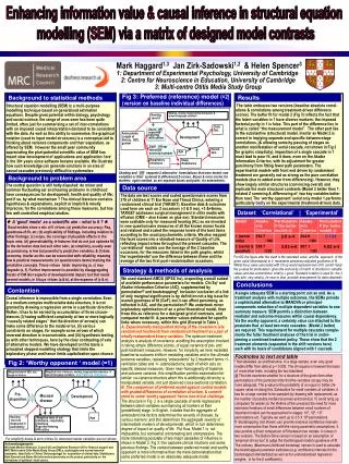
Enhancing information value & causal inference in structural equation modelling (SEM) via a matrix of designed model contrasts. Balance, anxiety, inappropriate behaviour, & speech/language variables. Hearing level #.

E N D
Enhancing information value & causal inference in structural equation modelling (SEM) via a matrix of designed model contrasts Balance, anxiety, inappropriate behaviour, & speech/language variables Hearing level # Weighted total of balance, anxiety, inappropriate behaviour, & speech/language variables ( and Parent & child QoL) Weighted total of SES, sex, length of history Child QoL ZsumOR reported hearing difficulties Antecedents: Length of history, SES, gender Development Pre- disposition Mucosal disease Development ZdiffOR ear Infection severity/number Parent QoL Age Age Hearing level as measured in audiometry ,Weighted total of ear infections, respiratory infections Reported hearing difficulties Respiratory infections Sleep disturbance Mark Haggard1,3 Jan Zirk-Sadowski1,2 & Helen Spencer3 1: Department of Experimental Psychology, University of Cambridge 2: Centre for Neuroscience in Education, University of Cambridge 3: Multi-centre Otitis Media Study Group Structural equation modelling (SEM) is a multi-purpose modelling technique based on generalised estimation equations. Despite great potential within biology, psychology and social science, the range of uses seen has been quite limited, often just for summarising a set of inter-correlations with an imposed causal interpretation declared to be consistent with the data. As well as this ability to summarise, the graphical notation (used to input model structures) is a conceptual aid to thinking about variance components and their separation, as offered by SEM. However the small peer community appreciating the pluri-potential scientific value of SEM has meant slow development of applications and application ‘lore’ in the 30+ years since software became available. We illustrate how such knowledge can generate solutions in an area of causal cascades previously difficult to systematise. The central question is still hotly disputed: do minor and common fluctuating ear and hearing problems in childhood have consequences for development, health and quality of life; and if so, by what mechanism ? The clinical literature contains hypotheses & explanations, explicit or implicit & mostly imprecise, for the correlations among these measures, but has few well-controlled empirical studies. Causal inference is impossible from a single correlation. Even in a medium-complex multivariable data structure, it is not granted by drawing a regression arrow in a particular direction. Rather, it has to be earned by accumulation of three circum-stances (i) having sufficient complexity at two or more logically “causally related stages” that the direction of arrow(s) can make some difference to the model error, (ii) various constraints on stages, for example some arrows of which reversed direction is inconceivable, and (iii) hypothesis testing as with other techniques, here by the clear contrasting of sets of alternative models. We have developed on this basis a principled stepped modelling strategy that limits the exploratory phase and hence limits capitalisation upon chance. Background to statistical methods Fig 3: Preferred (reference) model (=2) (version on baseline individual differences) Results The table embraces two versions (baseline absolute correl-ations & correlations among treatment-driven difference scores). The better fit for model 2 (Fig 3) reflects the fact that the latent variables in 1 have diverse markers; the imposed factorial purity in 1 is false. This part of the difference lies in what is called “the measurement model”. The other part lies in the substantive (structural) model. Insofar as Model 2 is correct in implying separate and specific between-stage correlations, (& allowing some by-passing of stages as another manifestation of serial cascade, not shown in Fig 3 for graphic simplicity), imposition of a single cascade in 1 must lead to poor fit, and it does, even on the Akaike Information Criterion, with its adjustment for greater parsimony from fitting fewer path parameters. The experimental models with front end driven by randomised treatment are generally not as strong as the pure correlation models (due to added error from differencing). However, they show largely similar structures (convincing overall) and replicate the main structural contrasts (Model 2 better than 1: rotated Z summing & differencing of two key variables better than raw.) The ‘worthy opponent’ serial only model 1 performs particularly badly on the experimental (treatment-driven) data. Shading and ‘OR’ separate 2 alternative formulations that were tested: raw variables or their summed & differenced Z-scores. Boxes & error circles for markers again omitted. as are separate boxes and paths for antecedents. Background to problem area Data source The data are test scores and scaled questionnaire scores from 376 of children at 11 Ear Nose and Throat Clinics, entering a randomised clinical trial (TARGET). Baseline data & outcomes used here are each on 2 occasions (-3 & 0 mo), +3 &+6mmo. TARGET addresses surgical management in otitis media with effusion (OME – also known as glue ear). Standard measures were available only for measured hearing (HL) so we invested in new questionnaire measures of all the known manor facets and retained and scaled the response levels of the best items according to the usual psychometric criteria. We also mapped the facet scores into a standard measure of Quality of Life, reflecting impact arises throughout the present cascades. The ‘correlational’ models use the average of the 2 baseline occasions, for the measures listed in the path graphs, whilst the ‘experimental’ use the difference between these and the average of the two first post-randomisation occasions. Dataset: ‘Correlational’ | ‘Experimental’ ♦ A ‘good’ model as a scientific aim – what is it ? ♦. Good models show a mix of 6 virtues: (a) predictive accuracy: Rsq, goodness-of-fit, etc; (b) explicability of findings, including relation to other findings; (c) scope, the coverage of plausible effects in the topic area; (d) generalisability, ie features that do not just optimise fit to the derivation data but suit other sets; (e) simplicity, usually seen as parsimony, ie few but powerful ly predictive variables; & (f) data economy, insofar as this can be reconciled with reliability, meaning few & practical measurements (or questionnaire items) marking the predictive concepts. These virtues trade: improving (a, c) may degrade (e, f). Further improvement is possible by disaggregating facets of OM &/or aspects of developmental impact, but that needs several models, ie it buys virtues (a & b), at the expense of (c & e). For AIC the figure after the slash is the saturated value, and the approach of the given value (downwards) to it represents parsimony-adjusted goodness of fit. Whilst the p-value associated with Ch-sq would represent lack of fit (small =bad) the p-value for permutation gives the exclusivity of match of structure to variable values and has conventional small p = good. Standard notation is used for the 3 cells with very small p. (ie near to best possible arrangement for data obtained/) Strategy & methods of analysis We used standard AMOS (SPSS Inc), inspecting a small subset of available performance parameters for models: Chi Sq* and Akaike Information Criterion (AIC), supplemented by permutation@ and bootstrapping#. Inclusion/ exclusion of a link of only marginal significance is by definition not a big issue for overall goodness of fit (GoF), but it can affect parsimony, as reflected in AIC, and the permutation P. We undertook minor exploratory optimisation of an a priori theoretical model, then froze this as reference for a designed grid of contrasts, and compared model fit & parameter values estimated for specific links where necessary, within this grid (Excerpt in Table ). A. Experimentally manipulated driving of the covariance (via randomised treatment) from randomised treatment as a pair of wholly independent binary variables. The optimum treatment analysis is analysis of covariance, avoiding the assumption involved in taking simple difference scores, of equal variance of pre- and post-treatment measures. However, for simplicity we here modelled baseline-to-outcome shifts in mediating variables and in the ultimate outcome variables, replacing “antecedents” by 2 treatment terms +/- ventilation tubes and +/- adenoidectomy, each of which acts on specific disease measures. Given near-homogeneity of baseline and outcome variance, this simplification permits examination for similar co-variance structure when this is additionally driven by a manipulated variable, not just observed cross-sectional correlation. B. The comparison of preferred model against control models with graded diffuseness of correlation structure, & commit-ment to some ‘worthy opponent’ hence non-trivial challenge. The structure in Fig 2 is a single cascade of serial regressions between latent variables summarising all markers at their (predefined) stage. In English, it states that the aggregate of antecedent risk factors determines the severity of disease, by various markers; and this determines the aggregate severity of intermediate markers of developmental, which in turn determines degree of impact on quality of life. Put thus, Model 1 is not implausible, but somewhat uninteresting and unimpressive. The more interesting postulate of two major cascades of influence is shown in Model 2, Fig 3; this captures clinical intuitions and some previous findings. The contest between preferred model and worthy opponent is more informative than the mere demonstration that some preferred model is an absolutely adequate model. Conclusions Contention A single adequate SEM is a starting point ,not an end. As a treatment analysis with multiple outcomes, the SEMs provide a sophisticated alternative to MANOVA or principal-components reduction of multiple dependent variables to one summary measure. SEM permits a distinction between mediator and outcome measures within causal dependency. Via the worthy opponent, a certainty value can attached to the postulate that at least two main cascades (Model 2 better) are required. This requirement for multiple cascades comple-ments the fuller treatment analyses of the trial in under-pinning a combined treatment policy. Those show that the 2 treatment elements (separated in the shift versions here) each with its basis of candidature aligned with 1 cascade. Footnotes to text and table * Not tabulated, as uninformative. In a large sample, even very good models differ from data at p < 0.005. The chi-square is however the basis of most other tests, including the two tabulated. @ This test examines whether for a structure of the given form other permutations of the particular slots that the variables occupy may be more adequate. The p-value is the probability of an equal or better chi-square value on doing this. Exhaustive for small numbers of variables, it has for a large number to be sampled (by drawing with replacement) as the number of possible models becomes astronomical. To avoid tying up computers for weeks (or the lifetime of the universe) the need for more extensive iterations of small differences between small numbers of important models can be approached in stages: 105, 106, 107 permutations etc. Typically we went up to 3.5 X 10⁶ permutations. # Bootstrapping (not shown) can provide empirical confidence intervals more conservative than those with the strong parametric assumptions. It also permits a direct comparison of fit between two models. It comes in two versions. The Bollen-Stine version is based on an assumption of ‘empirical-chi-sq test’ to judge the bootstrapped model’s goodness-of-fit. The ordinary (Maximum-Likelihood bootstrap) version is used to calculate the bootstrapped parameter estimates (e.g. confidence intervals for the bootstrapped standardized as well as for unstandardised regression weights, ie for the β coefficients). Fig 2: ‘Worthy opponent ‘ model (=1) For simplicity boxes & error circles for observed marker variables are not shown Acknowledgements We thank Medical Research Council UK and Deafness Research UK for financial support and MRC Multi-centre Otitis Media Study Group (ORLs, audiologists and nurses/research-assistants, listed fully in Clinical Otolaryngology) for acquisition of clinical data. Statisticians Kath Bennett and Elaine Nicholls worked previously on the project, particularly on the derivations of optimum facet scores,