Download
1 / 70
700 likes | 715 Vues
This research paper provides an overview and short review of visual inspection planning, discussing the issues and possible solutions. It focuses on determining optimal camera locations for inspecting geometric entities, minimizing measurement errors and the number of camera sensors needed.

E N D
Research directions on Visual Inspection Planning By Alexis H Rivera
Overview • Short review about visual inspection planning • Discussion of issues • Discussion of possible solutions and research directions
Visual Inspection Problem • Visual Inspection • Given an object, determine if it satisfies the design specification using camera as measurement tool • Visual Inspection Planning • Where should the camera be located to optimally inspect the desired geometricentities?
Visual Inspection Problem(cont.) • Optimality criterion • minimize the inherent measurement errors (quantization and displacement) • such that desired entities are: • resolvable • in focus • within field of view • visible • satisfy dimensional tolerances • minimize number of camera sensors needed
Visual Inspection Problem (cont.) • Finding optimal camera pose: • For a given set of entities, S • minimize F (tx, ty, tz, Φ, θ, Ψ, S) • subject to: • g1j <= 0 (resolution), for j=1 to k • g2a <= 0 (focus) • g2b <= 0 • g3 <= (field of view) • g4i <= 0 (visibility) for i=1 to m
Resolution • For each entity j, there is a constraint g1j() • Map smallest line entity to l pixels • Example: l = 2
Focus • Two constraints, g2a(), g2b() • Require closest and furthest entity vertices from the camera position to be within the far and near limits of the depth of field camera rf rc Far limit Near limit
Field Of View • One constraint: g3() • Bounding cone must be contained within the viewing cone Bounding cone Viewing cone
e1 e2 e4 e3 x y Visibility • Many equations: g4i() for i=1 to m • Plane equations that bound the visibility of the desired entities Example: To see entities e1, e2, e3, e4, the camera must satisfy equation y < 0
Visual Inspection Planning Solution: Finding optimal plan
Issues • The generation of the visibility constraints is incomplete • The software used to generate such constraints is obsolete • The current nonlinear optimization algorithm is very sensitive to the initial conditions • The process of generating a plan is not automated and is very tedious • The test cases used to validate the software were very simple
Possible Experiments • Optimization Process • Error Models • Inspection Planning Strategies
Possible Experiments (cont.) • Optimization Process • Alternative objective functions: Minimum Mean Square Error vs. Robustness Approach • Alternative optimization algorithm: Is there a better optimization algorithm? Does it matter? • Choice of initial pose Is it possible to find a good initial pose that guarantees an optimal solution?
Possible Experiments (cont.) • Error Models • Sub-pixel Quantization vs. Pixel Quantization, will it make a difference? • Inspection Planning Strategies • Characterizing sub-node strategies • Observations on more complicated objects • How to evaluate system? What criteria can be used to validate it?
Automation • How do I plan to automate this process?
Alternative objective functions • Idea: How does the objective function choice affects the inspection plan? • Explain straightforward objective function • Explain derivation of the MMSE • Explain robustness approach
Optimization Problem • Finding optimal camera pose: • For a given set of entities, S • minimize F (tx, ty, tz, Φ, θ, Ψ, S) • subject to: • g1j <= 0 (resolution), for j=1 to k • g2a <= 0 (focus) • g2b <= 0 • g3 <= (field of view) • g4i <= 0 (visibility) for i=1 to m
Optimization Problem • Different choices for objective function • (Tarabanis) Maximize weighted sum of sensor constraints • (Crosby) Minimize Mean Square Error • (Gu) Maximize the robustness • Objective function characterizes the quality of solution
Maximizing weighted sum of sensor constraints • Max F (tx, ty, tz, Φ, θ, Ψ, S) = α1g1+α2ag2a+α2bg2b+ α3g3+ α4g4 • The higher the value of the objective function the better the constraints are satisfied • Weights indicate how much a constraint contributes to the objective function
Maximizing weighted sum of sensor constraints • Issues: • Weights are based on experimental results • Optimization can be biased because of scaling issues • Assumption that multiple and couple objectives can be combines in an additive sense into a single objective
Minimizing Mean Square Error • Minimize the total expected error • Displacement errors • Quantization errors • MSE E[ε2]=E[εd2]+E[εq2]
Next Slides • Give a feel of the derivation of the MSE • Statistics are found defining and relating random variables • Some of this results are used in other objective function definitions
y v x z f u q p y z x Imaging process camera coordinate system image coordinate system World coordinate system
Imaging process • A point (x,y,z) in WCS is related to a point (u,v) in image plane coordinate by: u = Fu (x,y,z,tx, ty, tz, Φ, θ, Ψ) v = Fv(x,y,z, tx, ty, tz, Φ, θ, Ψ) • Fv, Fu, are coordinate transformation functions • (tx, ty, tz) vector representing camera location • (Φ, θ, Ψ) camera orientation
Imaging with displacement error • Let dx, dy, dz, dΦ, dθ, dΨ be displacement error in position and orientation • Assume I.I.D Gaussian random variables with zero mean and variance (σx2, σy2, σz2, σΦ2, σθ2, σψ2) • Mapping is now: u’ = Fu (x,y,z,tx, ty, tz, Φ, θ, Ψ, dx, dy, dx, dΦ, dθ, dΨ ) v’ = Fv(x,y,z, tx, ty, tz, Φ, θ, Ψ, dx, dy, dx ,dΦ, dθ, dΨ )
Displacement error of single point Image plane (u’,v’) εdu (u,v) εdv Displacement error for a each end point are new Gaussian RV εdu = u’ – u εdv = v’ – v
Displacement error of single point Displacement error for a each end point are new RV Let ξ χ ς be functions of the RVsdx, dy, dx, dΦ, dθ, dΨ These are Gaussian RVs Let εdu = u’ – u = ς / χ εdv = v’ – v = ξ / χ Then εdu and εdv are functions of the form g(x,y) = x/y The mean and variance can be approximated.
Displacement error of individual components of line Image plane (u’,v’) εdu2 εdu1 (u,v) εdv2 εdv1 Displacement error for a line are new RV εdx = εdu1 – εdu2 εdy = εdv1 – εdv2
Displacement error of line • Dimensional error is geometrically approximated: ddxcos() + dysin() = angle between line
Displacement error of k lines • Total dimensional error for k lines is:
Quantization Error 1D • Actual Length: L = lrx + u + v, where u,v uniform random variables • Quantized Length
Quantization Error 2D The actual and quantize length define new RVs
Quantization Error 2D The quantization error for the horizontal and vertical components:
Quantization Error for a line • Total quantization determined by geometric approximation, • qqxcos() + qysin() • zero mean • E[q 2]=σ q2 1/6(rx2cos2 + ry2sin2 )
Total quantization error for k lines Total dimensional error due to quantization in all lines:
Mean Square Error • Total error ε= εd – εq • MSE E[ε2]=E[εd2]+E[εq2]
Dimensional Tolerances • Dimensional Tolerance is satisfied if • fε(ε) is the probability density function of dimensional inspection error
Dimensional Tolerances • Can be rewritten in terms of characteristic equation • Where, • Φε(w)= Φεd(w) Φεq(w)
Finding Φεd(w) • Recall the following relations between the random variables • d = f(dx, dy) dxcos() + dysin() • εdx= f(du1, du2) = εdu1 – εdu2 • εdy = f(dv1, dv2) = εdv1 – εdv2 • εdu = f(ς, χ) = ς / χ • εdv = f(ξ, χ) = ξ / χ • Problem: We don’t know distribution of d because we don’t know distribution of εdu and εdv
Finding Φεd(w) • Solution: • Approximate distribution of εdu and εdv with Gaussian • It is shown that is an acceptable representation if camera pose if within feasible region
Finding Φεd(w) • Consequence • d is Gaussianbecause of linear relationships between RV
Finding Φεq(w) • Recall the following relations between the random variables • q = f(qx, qy) qxcos() + qysin() • εqx= f(Lqx, Lx) = Lqx – Lx • εdy = f(Lqy, Ly) = Lqy – Ly • f εqx(εqx) and f εqy(εqy) are triangular distributions defined in the range [-rx,rx] and [-ry,ry] respectively. Their characteristic function are:
Finding Φεq(w) • Finally Φεq(w) is given by:
Why do I care about all that derivation?? Next objective function: Robustness
Maximizing the robustness • Recall, • Define δ*2 as the maximum permissible inspection variance, > threshold δ*2 > δ = threshold δ*2 = δ -ΔL ΔL -ΔL ΔL