Data Analysis Essentials: Techniques, Tools, & Visualization for Effective Mining
Explore the fundamentals of Data Mining, from induction to deduction, accuracy to outliers, and handling errors & uncertainties. Learn how to manage data quality and make informed decisions through visualization and analysis. Enhance your understanding of various data types, including time-based, space-based, and image-based data. Gain insights into different types of analyses, propagation of errors, and reporting results accurately.

Data Analysis Essentials: Techniques, Tools, & Visualization for Effective Mining
E N D
Presentation Transcript
Data Analysis and Mining Peter Fox Data Science – ITEC/CSCI/ERTH-6961-01 Week 7, October 18, 2011
Reading assignment • Brief Introduction to Data Mining • Longer Introduction to Data Mining and slide sets • Software resources list • Data Analysis Tutorial • Example: Data Mining
Contents • Preparing for data analysis, completing and presenting results • Visualization as an information tool • Visualization as an analysis tool • New visualization methods (new types of data) • Managing the output of viz/ analysis • Enabling discovery • Use, citation, attribution and reproducability
Contents • Data Mining what it is, is not, types • Distributed applications – modern data mining • Science example • A specific toolkit set of examples (next week) • Classifier • Image analysis – clouds • Assignment 3 and week 7 reading • Week 8
Data types • Time-based, space-based, image-based, … • Encoded in different formats • May need to manipulate the data, e.g. • In our Data Mining tutorial and conversion to ARFF • Coordinates • Units • Higher order, e.g. derivative, average
Induction or deduction? • Induction: The development of theories from observation • Qualitative – usually information-based • Deduction: The testing/application of theories • Quantitative – usually numeric, data-based
‘Signal to noise’ • Understanding accuracy and precision • Accuracy • Precision • Affects choices of analysis • Affects interpretations (gigo) • Leads to data quality and assurance specification • Signal and noise are context dependent
Other considerations • Continuous or discrete • Underlying reference system • Oh yeah: metadata standards and conventions • The underlying data structures are important at this stage but there is a tendency to read in partial data • Why is this a problem? • How to ameliorate any problems?
Outlier • An extreme, or atypical, data value(s) in a sample. • They should be considered carefully, before exclusion from analysis. • For example, data values maybe recorded erroneously, and hence they may be corrected. • However, in other cases they may just be surprisingly different, but not necessarily 'wrong'.
Special values in data • Fill value • Error value • Missing value • Not-a-number • Infinity • Default • Null • Rational numbers
Errors • Three main types: personal error, systematic error, and random error • Personal errors are mistakes on the part of the experimenter. It is your responsibility to make sure that there are no errors in recording data or performing calculations • Systematic errors tend to decrease or increase all measurements of a quantity, (for instance all of the measurements are too large). E.g. calibration
Errors • Random errors are also known as statistical uncertainties, and are a series of small, unknown, and uncontrollable events • Statistical uncertainties are much easier to assign, because there are rules for estimating the size • E.g. If you are reading a ruler, the statistical uncertainty is half of the smallest division on the ruler. Even if you are recording a digital readout, the uncertainty is half of the smallest place given. This type of error should always be recorded for any measurement
Standard measures of error • Absolute deviation • is simply the difference between an experimentally determined value and the accepted value • Relative deviation • is a more meaningful value than the absolute deviation because it accounts for the relative size of the error. The relative percentage deviation is given by the absolute deviation divided by the accepted value and multiplied by 100% • Standard deviation • standard definition
Standard deviation • the average value is found by summing and dividing by the number of determinations. Then the residuals are found by finding the absolute value of the difference between each determination and the average value. Third, square the residuals and sum them. Last, divide the result by the number of determinations - 1 and take the square root.
Propagating errors • This is an unfortunate term – it means making sure that the result of the analysis carries with it a calculation (rather than an estimate) of the error • E.g. if C=A+B (your analysis), then ∂C=∂A+∂B • E.g. if C=A-B (your analysis), then ∂C=∂A+∂B! • Exercise – it’s not as simple for other calcs. • When the function is not merely addition, subtraction, multiplication, or division, the error propagation must be defined by the total derivative of the function.
Types of analysis • Preliminary • Detailed • Summary • Reporting the results and propagating uncertainty • Qualitative v. quantitative, e.g. see http://hsc.uwe.ac.uk/dataanalysis/index.asp
What is preliminary analysis? • Self-explanatory…? • Down sampling…? • The more measurements that can be made of a quantity, the better the result • Reproducibility is an axiom of science • When time is involved, e.g. a signal – the ‘sampling theorem’ – having an idea of the hypothesis is useful, e.g. periodic versus aperiodic or other… • http://en.wikipedia.org/wiki/Nyquist–Shannon_sampling_theorem
Detailed analysis • Most important distinction between initial and the main analysis is that during initial data analysis it refrains from any analysis. • Basic statistics of important variables • Scatter plots • Correlations • Cross-tabulations • Dealing with quality, bias, uncertainty, accuracy, precision limitations - assessing • Dealing with under- or over-sampling • Filtering, cleaning
Summary analysis • Collecting the results and accompanying documentation • Repeating the analysis (yes, it’s obvious) • Repeating with a subset • Assessing significance, e.g. the confusion matrix we used in the supervised classification example for data mining, p-values (null hypothesis probability)
Reporting results/ uncertainty • Consider the number of significant digits in the result which is indicative of the certainty of the result • Number of significant digits depends on the measuring equipment you use and the precision of the measuring process - do not report digits beyond what was recorded • The number of significant digits in a value infers the precision of that value
Reporting results… • In calculations, it is important to keep enough digits to avoid round off error. • In general, keep at least one more digit than is significant in calculations to avoid round off error • It is not necessary to round every intermediate result in a series of calculations, but it is very important to round your final result to the correct number of significant digits.
Uncertainty • Results are usually reported as result ± uncertainty (or error) • The uncertainty is given to one significant digit, and the result is rounded to that place • For example, a result might be reported as 12.7 ± 0.4 m/s2. A more precise result would be reported as 12.745 ± 0.004 m/s2. A result should not be reported as 12.70361 ± 0.2 m/s2 • Units are very important to any result
Secondary analysis • Depending on where you are in the data analysis pipeline (i.e. do you know?) • Having a clear enough awareness of what has been done to the data (either by you or others) prior to the next analysis step is very important – it is very similar to sampling bias • Read the metadata (or create it) and documentation
Tools • 4GL • Matlab • IDL • Ferret • NCL • Many others • Statistics • SPSS • Gnu R • Excel • What have you used?
Considerations for viz. as analysis • What is the improvement in the understanding of the data as compared to the situation without visualization? • Which visualization techniques are suitable for one's data? • E.g. Are direct volume rendering techniques to be preferred over surface rendering techniques?
Why visualization? • Reducing amount of data, quantization • Patterns • Features • Events • Trends • Irregularities • Leading to presentation of data, i.e. information products • Exit points for analysis
Types of visualization • Color coding (including false color) • Classification of techniques is based on • Dimensionality • Information being sought, i.e. purpose • Line plots • Contours • Surface rendering techniques • Volume rendering techniques • Animation techniques • Non-realistic, including ‘cartoon/ artist’ style
Compression (any format) • Lossless compression methods are methods for which the original, uncompressed data can be recovered exactly. Examples of this category are the Run Length Encoding, and the Lempel-Ziv Welch algorithm. • Lossy methods - in contrast to lossless compression, the original data cannot be recovered exactly after a lossy compression of the data. An example of this category is the Color Cell Compression method. • Lossy compression techniques can reach reduction rates of 0.9, whereas lossless compression techniques normally have a maximum reduction rate of 0.5.
Remember - metadata • Many of these formats already contain metadata or fields for metadata, use them!
Tools • Conversion • Imtools • GraphicConverter • Gnu convert • Many more • Combination/Visualization • IDV • Matlab • Gnuplot • http://disc.sci.gsfc.nasa.gov/giovanni
New modes • http://www.actoncopenhagen.decc.gov.uk/content/en/embeds/flash/4-degrees-large-map-final • http://www.smashingmagazine.com/2007/08/02/data-visualization-modern-approaches/ • Many modes: • http://www.siggraph.org/education/materials/HyperVis/domik/folien.html
Publications, web sites • www.jove.com - Journal of Visualized Experiments • www.visualizing.org - • logd.tw.rpi.edu -
Managing visualization products • The importance of a ‘self-describing’ product • Visualization products are not just consumed by people • How many images, graphics files do you have on your computer for which the origin, purpose, use is still known? • How are these logically organized?
(Class 2) Management • Creation of logical collections • Physical data handling • Interoperability support • Security support • Data ownership • Metadata collection, management and access. • Persistence • Knowledge and information discovery • Data dissemination and publication
Use, citation, attribution • Think about and implement a way for others (including you) to easily use, cite, attribute any analysis or visualization you develop • This must include suitable connections to the underlying (aka backbone) data – and note this may not just be the full data set! • Naming, logical organization, etc. are key • Make them a resource, e.g. URI/ URL
Producability/ reproducability • The documentation around procedures used in the analysis and visualization are very often neglected – DO NOT make this mistake • Treat this just like a data collection (or generation) exercise • Follow your management plan • Despite the lack or minimal metadata/ metainformation standards, capture and record it • Get someone else to verify that it works
Data Mining – What it is • Extracting knowledge from large amounts of data • Motivation • Our ability to collect data has expanded rapidly • It is impossible to analyze all of the data manually • Data contains valuable information that can aid in decision making • Uses techniques from: • Pattern Recognition • Machine Learning • Statistics • High Performance Database Systems • OLAP • Plus techniques unique to data mining (Association rules) • Data mining methods must be efficient and scalable
Data Mining – What it isn’t • Small Scale • Data mining methods are designed for large data sets • Scale is one of the characteristics that distinguishes data mining applications from traditional machine learning applications • Foolproof • Data mining techniques will discover patterns in any data • The patterns discovered may be meaningless • It is up to the user to determine how to interpret the results • “Make it foolproof and they’ll just invent a better fool” • Magic • Data mining techniques cannot generate information that is not present in the data • They can only find the patterns that are already there
Data Mining – Types of Mining • Classification (Supervised Learning) • Classifiers are created using labeled training samples • Training samples created by ground truth / experts • Classifier later used to classify unknown samples • Clustering (Unsupervised Learning) • Grouping objects into classes so that similar objects are in the same class and dissimilar objects are in different classes • Discover overall distribution patterns and relationships between attributes • Association Rule Mining • Initially developed for market basket analysis • Goal is to discover relationships between attributes • Uses include decision support, classification and clustering • Other Types of Mining • Outlier Analysis • Concept / Class Description • Time Series Analysis
Science Motivation • Study the impact of natural iron fertilization process such as dust storm on plankton growth and subsequent DMS production • Plankton plays an important role in the carbon cycle • Plankton growth is strongly influenced by nutrient availability (Fe/Ph) • Dust deposition is important source of Fe over ocean • Satellite data is an effective tool for monitoring the effects of dust fertilization
Hypothesis • In remote ocean locations there is a positive correlation between the area averaged atmospheric aerosol loading and oceanic chlorophyll concentration • There is a time lag between oceanic dust deposition and the photosynthetic activity
Primary source of ocean nutrients OCEAN UPWELLING WIND BLOWNDUST SAHARA SEDIMENTS FROM RIVER
CLOUDS Factors modulating dust-ocean photosynthetic effect SST CHLOROPHYLL DUST NUTRIENTS SAHARA
Objectives • Use satellite data to determine, if atmospheric dust loading and phytoplankton photosynthetic activity are correlated. • Determine physical processes responsible for observed relationship
Data and Method • Data sets obtained from SeaWiFS and MODIS during 2000 – 2006 are employed • MODIS derived AOT • SeaWIFS • MODIS • AOT
The areas of study *Figure: annual SeaWiFS chlorophyll image for 2001 8 7 6 1 2 5 3 4 1-Tropical North Atlantic Ocean 2-West coast of Central Africa 3-Patagonia 4-South Atlantic Ocean 5-South Coast of Australia 6-Middle East 7- Coast of China 8-Arctic Ocean
Tropical North Atlantic Ocean dust from Sahara Desert -0.17504 -0.0902 -0.328 -0.4595 -0.14019 -0.7253 -0.1095 Chlorophyll AOT -0.68497 -0.15874 -0.85611 -0.4467 -0.75102 -0.66448 -0.72603