This research was supported by HEI 4746-RFA05-2/06-7.

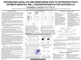
1. CAR space-time process (4 km grid, daily or monthly in time) weather, GIS info interpolated to 4 km grid Latent space-time structure Latent PM2.5 on 4 km grid (daily or monthly) Weather (PBL, RH) and space-time calibration Within-grid cell covariates Likelihood portion of model MODIS AOD, 10:30 am GOES AOD, avg of half-hour obs. MISR AOD, 10:30 am 24hr avg PM2.5 PM2.5 likelihood AOD likelihoods INTEGRATING SATELLITE AND MONITORING DATA TO RETROSPECTIVELY ESTIMATE MONTHLY PM2.5 CONCENTRATIONS IN THE EASTERN U.S. Christopher J. Paciorek1 and Yang Liu2 1Department of Biostatistics, Harvard School of Public Health, Boston, MA; 2Department of Environmental Health, Harvard School of Public Health, Boston, MA www.biostat.harvard.edu/~paciorek/research/presentations/presentations.html DATA SOURCES STATISTICAL MODELLING INTRODUCTION • Remote sensing observations of aerosol hold promise for adding information about PM2.5 concentrations beyond that from monitors, particularly in suburban and rural areas with limited monitoring. • AOD (aerosol optical depth) observations are frequently missing, and noisy and biased relative to PM2.5. • Bayesian statistical modeling holds promise for integrating AOD, PM2.5, and GIS and weather information to predict monthly PM2.5 concentrations on a fine grid (4 km). • Key challenges include: • 1.) formulation of a statistical model to relate observations to a latent space-time process representing true PM2.5 in a way that accounts for spatial and temporal mismatch and nature of error and bias. • 2.) representation of the latent process that provides appropriate spatial and temporal correlation while allowing for computationally-efficient statistical estimation Basic solutions: • Calibrate AOD to PM2.5 (partly as preprocessing, partly in model) • Relate all quantities to latent PM2.5 variable on base 4km grid • Treat AOD at natural resolution, as weighted averages of PM2.5 on base grid, with calibration • Use conditional autoregressive (CAR) space-time statistical models to build space-time correlation in computationally feasible manner (use weights decaying with distance to ensure adequate spatial correlation) • Use weather and GIS information to help estimate PM2.5 Challenges: • Large data sources and desire for fine-scale prediction • AOD is a biased and noisy reflection of PM2.5 • Need for spatial and temporal correlation in modelling PM2.5 • Spatial correlation of AOD errors • Irregular sampling of both AOD and PM2.5 in space and time • Missingness of AOD may be related to PM2.5 levels • Spatial mismatch of data sources (point data plus varying areal units) Remote Sensing Observations PM2.5 and Covariate Information • MISR AOD: 16 day orbit repeat, observations every 4-7 days at 10:30 am for a given location, 17.6 km resolution • MODIS AOD: 16 day orbit repeat, observations every 1-2 days for a given location, 10 km resolution • GOES AOD: observations every half hour, 4 km resolution SUMMARY OF INTERIM RESULTS • PM2.5 measurements from AQS and IMPROVE: daily average, every 1, 3, or 6 days • Weather data at 32 km, 3 hour resolution from North American Regional Reanalysis • GIS-derived information: distance to roads by road class, population density, land use • Daily MISR AOD shows little association with ground monitors of PM2.5 across time and at individual stations. • Calibration of MISR AOD to PM2.5 measurements, modified by weather variables and spatial and temporal bias terms, improves correlations between AOD and PM2.5, particularly when averaging over time. • There is limited evidence that missing MISR AOD observations are associated with the level of PM2.5. • Satellite AOD holds some promise for enhancing predictions of PM2.5, but is likely most useful at monthly or yearly temporal scale. • Ability of satellite AOD to improve predictions relative to models based on PM2.5 data, weather and GIS variables is a key question. • Conditional autogregressive (CAR) space-time models hold promise for computationally efficient latent process estimation in a Bayesian statistical framework. • CAR models can account for spatial and temporal correlation induced by underlying physical reality, areally-integrated satellite observations, and time averaging of incomplete satellite observations. ASSESSMENT AND CALIBRATION OF MISR AOD Calibration and temporal averaging improve the relationship AOD not strongly related to daily PM Longitudinal association: four fixed sites across days Likelihood Terms Latent Process Representation and Fitting Cross-sectional association: four fixed days across sites Scatterplots of AOD against PM across site for four individual days (top row) and for AOD against PM across time for four individual sites (bottom row) suggest that at the daily scale and without calibration, the association is weak and variable. Log AOD vs. PM before and after calibration with RH, PBL, and spatial and temporal bias terms (top row). Average calibrated log AOD against average PM over a month and over a year (bottom row). ONGOING AND NEAR-TERM WORK Statistical calibration of AOD to PM Missingness bias? GAM model: Calibration: • Calibration of GOES and MODIS AOD observations with PM2.5, modified by weather variables and spatial and temporal bias terms. • Comparison of strength of association of AOD with PM2.5 for the different satellite instruments. • Assessment of spatial and temporal scales at which satellite AOD is useful for estimating PM2.5. • Ongoing data processing and matching of satellite observations and GIS variables to base 4 km grid. • Full development of daily- and monthly-scale Bayesian statistical models for PM2.5 prediction based on CAR framework. • Initial model fitting for small region and several month time period to assess computational feasibility and compare daily/monthly approaches. Build Model at Daily or Monthly Level? Build Model at Daily or Monthly Level? Daily model • More naturally treats daily observations • Satellite pixels represented as weighted averages of 4 km grid cells • PM2.5 data relatively sparse • Much more computationally intensive • Monthly latent PM2.5 estimated as average of latent daily estimates on grid Monthly model • Aggregate data to the month after daily satellite calibration; more computationally feasible • Need to assign AOD measurements to multiple 4 km cells and then average within cells • AOD and PM2.5 monthly averages do not have constant error variance (varying number of days) • Unusual induced correlations of time-averaged AOD. Relationships of log(AOD) with PM as modified by time, space, log(PBL), and RH. Smooth terms indicate how each factor affects the bias in log(AOD) as a proxy for PM. For example during the summer (days 150-240), log(AOD) is more positively offset (biased) with respect to PM than in the winter. GAM provides calibration of log(AOD) at daily scale that allows averaging to longer time periods. After adjustment for space, time, and PBL, there is some evidence that missing AOD indicates lower (~2 ug/m3) PM in summer and higher (0.67 ug/m3) PM in fall, with little difference in winter and spring. This research was supported by HEI 4746-RFA05-2/06-7.