Edgar G. Pavia CICESE, Ensenada, B.C., Mexico epavia@cicese.mx

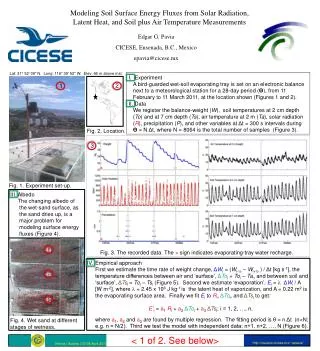
1. Modeling Soil Surface Energy Fluxes from Solar Radiation, Latent Heat, and Soil plus Air Temperature Measurements Edgar G. Pavia CICESE, Ensenada, B.C., Mexico epavia@cicese.mx Lat: 31° 52' 09" N. Long: 116° 39' 52" W. Elev: 66 m above msl. I. Experiment A bird-guarded wet-soil evaporating tray is set on an electronic balance next to a meteorological station for a 28-day period (Θ), from 11 February to 11 March 2011, at the location shown (Figures 1 and 2). II. Data We register the balance-weight (W), soil temperatures at 2 cm depth (To) and at 7 cm depth (Ts), air temperature at 2 m (Ta), solar radiation (R), precipitation (P), and other variables at Δt = 300 s intervals during Θ = N Δt, where N = 8064 is the total number of samples (Figure 3). 2 1 Fig. 2. Location. 3 N W E S × × Fig. 1. Experiment set-up. III. Albedo The changing albedo of the wet-sand surface, as the sand dries up, is a major problem for modeling surface energy fluxes (Figure 4). × × Fig. 3. The recorded data. The × sign indicates evaporating-tray water recharge. 4a • Empirical approach • First we estimate the time rate of weight change, ΔWi= (Wi-½ – Wi+½ ) / Δt [kg s-1],the temperature differences between air and ‘surface’, ΔToi = Toi – Tai, and between soil and ‘surface’, ΔTsi= Toi – Tsi(Figure 5). Second we estimate ‘evaporation’, Ei =  ΔWi/ A [W m-2], where  = 2.45 x 106 J kg-1 is the latent heat of vaporization, andA = 0.22 m2 is the evaporating surface area. Finally we fit Eito Ri, ΔToi, and ΔTsi to get: • E’i = a1Ri + a2ΔToi + a3ΔTsi; i = 1, 2, …, n, • where a1, a2anda3 are found by multiple regression. The fitting period is θ = n Δt (n<N; e.g. n = N/2). Third we test the model with independent data: n+1, n+2, …, N (Figure 6). 4b 4c Fig. 4. Wet sand at different stages of wetness. < 1 of 2. Seebelow> Vienna | Austria | 03-08 April 2011 http://usuario.cicese.mx/~epavia/

2. < Two > Vienna | Austria | 03-08 April 2011 < 2 of 2. Seeabove> http://www.cicese.edu.mx/ • Method (briefreview) • Makethe vector: • y = [E1E2 … En] • and thematrix: • R11R21 … Rn1 • X = ΔTo12ΔTo22 ... • ΔTs13ΔTs23 … ΔTsn3. • Withthe vector of coefficients (to be found): • a = [a1 a2 a3] • theproblembecomes: • y’ =aX. • Minimizing • Q = (y – aX) (y – aX)T • i.e. ∂Q/∂a = 0 • yields • a = yXT(XXT)-1 • and thus • y' = [E’1E’2 … E’n]. • Next, test aforstabilitywiththeindependent data: • (Ri, ΔToi, ΔTsi), i = n+1, n+2, …, N, • toobtain: • E’n+1, E’n+2, … E’N. • If, in addition, a1 < 1,a2 < 0,and a3 < 0, themodelisstable and ‘physical’. 0.05 5 ΔW (per Δt)[Kg] Kg 0 ΔTo [C] -0.05 ΔTs [C] Fig. 5. Weight difference in a 5-minute interval (ΔW), air to surface temperature difference (ΔTo), and soil to surface temperature difference (ΔTs). 6 ∙ Ei=ΔWi/ A; i = 1, 2, …, N. ∙ E’i = a1Ri + a2ΔToi+ a3ΔTsi ; i = 1, 2, …, N. × × + + + + a1 = 0.41 a2 = -3.30 [W m-2 C-1] a3 = -9.88 [W m-2 C-1] Fig. 6. Estimated (E) and modeled ‘evaporation’ (E’). The + sign indicates recorded precipitation (see Figure 3). 100 % 0 10 0 m/s 0 Fig. 7. Relative humidity (yellow) and wind speed (bluish). VI. Conclusions The empirical model works relatively well, with correlation coefficient r(E, E’) = 0.9, for the entire 28-d observing period (N = 8064). Obviously it cannot simulate heavy-precipitation events nor anomalously dry and windy conditions (see Figures 6 and 7). Evaporation depends strongly on solar radiation (R), since the temperature-difference terms (ΔToand ΔTs) contribute with minimum variance explained. However these latter terms do not render the model unstable when modeling independent data (Figure 6, red line), and their coefficients, obtained by the multiple regression method, allow us to optimistically model the simplified surface energy flux balance: Rn + H + G – E= 0, if the net radiation Rn ~ a1R, the sensible heat flux H ~ a2ΔTo, and the surface soil heat flux G ~ a3ΔTsi.