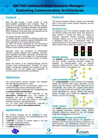
Download
1 / 41
410 likes | 563 Vues
Flexible wireless communication architectures. Sridhar Rajagopal Department of Electrical and Computer Engineering Rice University, Houston TX Faculty Candidate Seminar – Southern Methodist University April 23, 2003. This work has been supported in part by NSF, Nokia and Texas Instruments.

E N D
Flexible wireless communication architectures Sridhar Rajagopal Department of Electrical and Computer Engineering Rice University, Houston TX Faculty Candidate Seminar – Southern Methodist University April 23, 2003 This work has been supported in part by NSF, Nokia and Texas Instruments
Wireless Cellular Bluetooth/ Home Networks Wireless LAN Future wireless devices demand flexibility • Multiple algorithms and environments supported in same device • High data rate mobile devices with multimedia • Flexible algorithms: Multiple antennas, complex signal processing • Flexible architectures: High performance (Mbps), low power (mW) • Fast design with structured exploration
Flexible Algorithms Mapping Flexible Architectures Flexibility needed in different layers Application Layer Puppeteer project at Rice http://www.cs.rice.edu/CS/Systems/Puppeteer/ Network Layer MAC Layer Physical Layer Analog RF
Algorithms: Flexibility: support variety of sophisticated algorithms Architectures: Flexibility: adapts hardware to algorithms Fast, structured design exploration Design me Research vision: Attain flexibility
Contributions: Algorithms Multi-user channel estimation:[Jnl. Of VLSI Sig. Proc.’02, ASAP’00] • Matrix-inversions • Numerical techniques • conjugate-gradient descent for complexity reduction Multi-user detection: [ISCAS’01] • Block-based computation to streaming computations • Pipelining, lower memory requirements Parallel, fixed-point, streaming VLSI implementations [IEEE Trans. Wireless Comm.’02]
Contributions: Architectures Heterogeneous DSP-FPGA system designs: [ICSPAT’00] Computer arithmetic:[Symp. On Comp. Arith’01] Dynamic truncation in ASICs using on-line arithmetic with Most Significant Digit First computation [Ph.D. Thesis] Scalable Wireless Application-specific Processors (SWAPs) Rapid, structured architectures with flexibility-performance tradeoffs
+ + + + … ? ? ? ? * * * * * * * * Scalable Wireless Application-specific Processors • Family of flexible programmable processors • Clusters of ALUs • High performance by supporting 100’s of ALUs • Can provide customization for various algorithms • Adapts (“swaps”) architecture dynamically for power Scale ALUs Scale Clusters
+ + + + … ? ? ? ? * * * * * * * * Rapid, structured design for SWAPs Low “complexity”, parallel, fixed point algorithms Architecture Exploration ASIC design apply SWAPs DSP design apply
Research vision summary • Provide a structured framework to rapidly explore: • flexible, high performance, low power architectures (SWAPs) • Efficient algorithm design for mapping to SWAPs • Understanding of algorithms, DSPs and ASICs used • Flexibility-performance trade-offs Inter-disciplinary research: Wireless communications, VLSI Signal Processing, Computer architecture, Computer arithmetic, Circuits, CAD, Compilers
Talk Outline • Research vision • SWAPs - Background • Algorithm design for SWAPs • Architecture design for SWAPs • Current and Future Research Goals
1 ALU RF 4 16 32 Register File SWAPs borrow from DSPs • DSPs use : Instruction Level Parallelism (ILP) Subword Parallelism (MMX) • Not enough ALUs for GOPs of computation-- Need 100’s • TI C6x has 8 ALUs • Why not more ALUs? • Cannot support more registers (area,ports) • Difficult to find ILP as ALUs increase
SWAPs borrow from ASICs Exploit data parallelism (DP) • Available in many wireless algorithms • This is what ASICs do! int i,a[N],b[N],sum[N]; // 32 bits short int c[N],d[N],diff[N]; // 16 bitspacked for (i = 0; i< 1024; ++i) { sum[i] = a[i] + b[i]; diff[i] = c[i] - d[i]; } DP ILP Subword
Kernel Stream Input Data Output Data Interference Cancellation Viterbi decoding receivedsignal Matched filter Decoded bits Correlator channel estimation SWAPs borrow from stream processors • Kernels (computation) and streams (communication) • Use local data in clusters providing GOPs support • Imagine stream processor at Stanford [Rixner’01] Scott Rixner. Stream Processor Architecture, Kluwer Academic Publishers: Boston, MA, 2001.
Internal Memory + + ILP + * * * SWAPs are multi-cluster DSPs Memory: Stream Register File (SRF) + + + + + + + + … ILP + + + + * * * * * * * * * * * * DP SWAPs adapt clusters to DP Identical clusters, same operations. Power-down unused FUs, clusters DSP (1 cluster)
SRF Arithmetic clusters in SWAPs Distributed Register Files (supports more ALUs) From/To SRF + + + + + + * * + + * * Cross Point / Intercluster Network / / / Comm. Unit Scratchpad (indexed accesses)
Talk Outline • Research vision • SWAPs Background • Algorithm design for SWAPs • Architecture design for SWAPs • Current and Future Research Goals
SWAPs: Physical layer algorithms Antenna Baseband processing Detection Decoding Higher (MAC/Network/OS) Layers RF Front-end Channel estimation Complex signal processing algorithms with GOPs of computation
SWAP mapping example: Viterbi decoding • Multiple antenna systems (MIMO systems) • Complexity exponential with transmit x receive antennas • Estimation: Linear MMSE, blind, conjugate gradient…. • Detection: FFT, (blind) interference cancellation…. • Decoding: Viterbi, Turbo, LDPC…. & joint schemes • SWAP flexibility lets you use the best algorithms for the situation Example for concept demonstration: Viterbi decoding
Parallel Viterbi Decoding for SWAPs ACS Unit Traceback Unit Decoded bits Detected bits • Add-Compare-Select (ACS) : trellis interconnect : computations • Parallelism depends on constraint length (#states) • Traceback: searching • Conventional • Sequential (No DP) with dynamic branching • Difficult to implement in parallel architecture • Use Register Exchange (RE) • parallel solution
ACS in SWAPs Regular ACS DP vector X(0) X(0) X(0) X(0) X(1) X(2) X(1) X(1) X(2) X(4) X(2) X(2) X(3) X(6) X(3) X(3) X(4) X(4) X(4) X(8) X(5) X(10) X(5) X(5) X(12) X(6) X(6) X(6) X(14) X(7) X(7) X(7) X(8) X(8) X(8) X(1) X(9) X(9) X(9) X(3) X(5) X(10) X(10) X(10) X(7) X(11) X(11) X(11) X(12) X(12) X(12) X(9) X(13) X(11) X(13) X(13) X(14) X(13) X(14) X(14) X(15) X(15) X(15) X(15) Parallel Viterbi needs re-ordering for SWAPs Exploiting Viterbi DP in SWAPs: • Use RE instead of regular traceback • Re-order ACS, RE
Talk Outline • Research vision • SWAP Background • Algorithm design for SWAPs • Architecture design for SWAPs • Current and Future Research Goals
SWAP architecture design More clusters better than more ALUs/per cluster (if #clusters > 2) • Decide how many clusters • Exploit DP • Decide what to put within each cluster • Maximize ILP with high functional unit efficiency • Search design space with “explore” tool Time-power-area characterization + + + + … ? ? ? ? ILP * * * * * * * * DP
(80,34) (85,24) (85,17) 160 (85,13) 140 (85,11) (70,59) 120 (73,41) 100 (62,62) Instruction count (76,33) 80 (72,22) (65,45) (54,59) (43,58) (72,19) (47,43) (61,33) 60 (39,41) (60,26) (49,33) 40 (61,22) (40,32) (48,26) 1 1 (39,27) (50,22) 2 2 (39,22) 3 3 #Multipliers #Adders 4 4 5 5 Design a SWAP cluster: “Explore” Auto-exploration of adders and multipliers for “ACS" (Adder util%, Multiplier util%)
“Explore” tool benefits • Instruction count vs. ALU efficiency • What goes inside each cluster • Design customized application-specific units • Better performance with increased ALU utilization • Explore multiple algorithms • turn off functional units not in use for given kernel • Vdd-gating, clock gating techniques
Example for SWAP architecture design DP Explore Algorithm 1 : 3 adders, 3 multipliers, 32 clusters Explore Algorithm 2 : 4 adders, 1 multiplier, 64 clusters Explore Algorithm 3 : 2 adders, 2 multipliers, 64 clusters Explore Algorithm 4 : 2 adders, 2 multipliers, 16 clusters Chosen Architecture: 4 adders, 3 multipliers, 64 clusters ILP
SWAP flexibility provides power savings • Multiple algorithms • Different ALU, cluster requirements • Turning off ALUs ( –add –mul compiler options) • Use the right #ALUs from “explore” tool • Turning off clusters • Data across SRF of all clusters • Cluster only has access to its own SRF • Next kernel may need data from SRF of other clusters • Reconfiguration support needs to be provided
SWAPs provide cluster reconfiguration SRF Mux-Demux Network With Stream buffers Clusters Additional latency (few cycles) due to microcontroller stalls - Minimal loss in performance
Cluster reconfiguration for Viterbi DP Can be turned OFF Packet 1 Constraint length 7 (16 clusters) Packet 2 Constraint length 9 (64 clusters) Packet 3 Constraint length 5 (4 clusters)
Execution Time (cycles) SWAPs provide flexibility at negligible overhead Clusters Memory 64-bit Rate ½ Packet 1 K = 7 Kernels (Computation) No Data Memory accesses Packet 2 K = 9 Packet 3 K = 5
SWAP exploration for Viterbi decoding 1000 K = 9 K = 7 Different SWAPs (Without reconfiguration) DSP K = 5 Same SWAP (With reconfiguration) 100 Frequency needed to attain real-time (in MHz) 10 Max DP 1 1 10 100 Number of clusters Ideal C64x (w/o co-proc) needs ~200 MHz for real-time
SWAPs : Salient features • 1-2 orders of magnitude better than a DSP • Any constraint length 10 MHz at 128 Kbps • Same code for all constraint lengths • no need to re-compile or load another code • as long as parallelism/cluster ratio is constant • Power savings due to dynamic cluster scaling
Viterbi Clusters Used Peak Power K = 9 64 ~90 mW K = 7 16 ~28.57 mW K = 5 4 ~13.8 mW overhead 0 ~8.1 mW 90 80 70 60 50 Power (in mW) 40 30 20 10 0 0 10 20 30 40 50 60 70 Active Clusters (max 64) Expected SWAP power consumption • Power model based on [Khailany’03] • 64 clusters and 1 multiplier per cluster: • 0.13 micron, 1.2 V • Peak Active Power: ~9 mW at 1 MHz (DSP ~1 mW) • Area: ~53.7 mm2 • 10 MHz, 128 Kbps with reconfiguration DSP, K = 9 1 ~200 mW Exploring the VLSI Scalability of Stream Processors, Brucek Khailany et al, Proceedings of the Ninth Symposium on High Performance Computer Architecture, February 8-12, 2003
100000 FAST MEDIUM DSP SLOW 10000 32-user base-station 1000 Frequency needed to attain real-time (in MHz) 100 Mobile 10 100 1 10 Number of clusters Multiuser Estimation-Detection+Decoding Real-time target : 128 Kbps per user Fading scenarios Ideal C64x (w/o co-proc) needs ~15 GHz for real-time
Expected SWAP power : base-station • 32 user base-station with 3 X’s per cluster and 64 clusters: • 0.13 micron, 1.2 V • Peak Active Power: ~18.19 mW for 1 MHz (increased X) • Area: ~93.4 mm2 • Total Peak Base-station power consumption: • ~18.19 W at 1 GHz for 32 users at 128 Kbps/user
Talk Outline • Research vision • SWAP Background • Algorithm design for SWAPs • Architecture design for SWAPs • Current and Future Research Goals
Current research: Flexibility vs. performance SWAPs: 128 Kbps at ~10-100 mW for Viterbi • Borrow DP from ASICs! • suitable for base-stations • Flexibility more important than power • suitable for mobile devices • Power constraints tighter • can be customized for further power savings Handset SWAPs (H-SWAPs) • Borrow Task pipelining from ASICs! • Application-specific units and specialized comm. network
SRF + + + + + + + + + + + + + + + + + + + + + + + + + + + + + + + + + + + + + + + + + * + + * * + + + * + + + + + + + + + + + + … * * * * * * * * + + + + + + + + + * * * * * * * * * * * * * * * * * * Limited DP Limited DP Limited DP * * * * * * * * * Limited DP DP H-SWAPs (collection of customized SWAPlets) SWAPlet (limit clusters) Handset SWAPs: H-SWAPs • Trade Data Parallelism for Task Pipelining SWAPs (max. clusters and reconfigure)
Sample points in architecture exploration Programmable solutions with increased customization DSPs (1 cluster) SWAPs (multiple) H-SWAPs (optimized for handsets) ILP Subword DP Task Pipelining Custom ALUs ILP Subword DP ILP Subword Performance, Power benefits (with decreasing flexibility)
Future: Efficient algorithms and mapping Multiple antenna systems with 1-2 orders-of-magnitude higher complexity
Future research: Architectures Generalized and structured framework and tools • Joint algorithm-architecture exploration • Area-time-power-flexibility tradeoffs Potential applications: embedded systems • Image and Video processing: • Cameras : variety of compression algorithms • Biomedical applications: • Hearing aids: DSP running on body heat* • Sensor networks • Compression of data before transmission *Quote: Gene Frantz, TI Fellow
SWAPs: Flexibility, Performance, Power • Need flexibility in future wireless devices • Algorithms and Architectures • Rapid Exploration for Scalable, Wireless Application-specific Processors • Structured approach with flexibility-performance trade-offs • SWAPs - flexibility, high performance and low power • Exploit data parallelism like ASICs • 1-2 orders better performance than DSPs • Turn off unused clusters and unused ALUs for low power