LAPS Technical Overview
LAPS Technical Overview. LAPS Mission. A system designed to: Exploit all available data sources Create analyzed and forecast grids with analysis systems and numerical models Build products for specific forecast applications Provide reliable forecast guidance Use advanced display technology

LAPS Technical Overview
E N D
Presentation Transcript
LAPS Mission A system designed to: • Exploit all available data sources • Create analyzed and forecast grids with analysis systems and numerical models • Build products for specific forecast applications • Provide reliable forecast guidance • Use advanced display technology …All within a local weather office, forward site, or in fully deployed mode
Univariate Analysis Analysis Merging/ Balancing NWP Model Initialization/ Prediction Data LAPS Basic Structure Very diverse Force geometric, Reconcile gridded Generate forecasts data sets smoothing constraints fields; force and user-specific to interpolate data to consistency based products high resolution grids on atmospheric scale
LAPS Components - Stage 1 • Data Acquisition and Quality Control • Univariate Analysis of the Following Fields • Temperature • Winds • Water Vapor • Clouds • Microphysical variables • Vertical motions
Data Acquisition and Quality ControlLAPS supports a wide range of data types
Multi-layered Quality Control • Gross Error Checks • RoughClimatologicalEstimates • Station Blacklist • Dynamical Models • Use of background and mesoscale models • Standard Deviation Check • Statistical Models • Buddy Checking
Standard Deviation Check • Compute Standard Deviation of observations-background • Remove outliers • Now adjustable via namelist
Remapping Strategy • Polar to Cartesian • 2D or 3D result (narrowband / wideband) • Average Z,V of all gates directly illuminating each grid box • QC checks applied • Typically produces sparse arrays at this stage
Remapping Strategy (reflectivity) • Horizontal Analysis/Filter (Reflectivity) • Needed for medium/high resolutions (<5km) at distant ranges • Replace unilluminated points with average of immediate grid neighbors (from neighboring radials) • Equivalent to Barnes weighting at medium resolutions (~5km) • Extensible to Barnes for high resolutions (~1km) • Vertical Gap Filling (Reflectivity) • Linear interpolation to fill gaps up to 2km • Fills in below radar horizon & visible echo
Mosaic Strategy (reflectivity) • Nearest radar with valid data used • +/- 10 minute time window • Final 3D reflectivity field produced within cloud analysis • Wideband is combined with Level-III (NOWRAD/NEXRAD) • Non-radar data contributes vertical info with narrowband • QC checks including satellite • Help reduce AP and ground clutter
Surface Precipitation Accumulation • Algorithm similar to NEXRAD PPS, but runs in Cartesian space • Rain / Liquid Equivalent • Z = 200 R ^ 1.6 • Snow case: use rain/snow ratio dependent on column maximum temperature • Reflectivity limit helps reduce bright band effect
Future Cloud / Radar analysis efforts • Account for evaporation of radar echoes in dry air • Sub-cloud base for NOWRAD • Below the radar horizon for full volume reflectivity • Continue adding multiple radars and radar types • Evaluate Ground Clutter / AP rejection
Future Cloud/Radar analysis efforts (cont) • Consider Terrain Obstructions • Improve Z-R Relationship • Convective vs. Stratiform • Precipitation Analysis • Improve Sfc Precip coupling to 3D hydrometeors • Combine radar with other data sources • Model First Guess • Rain Gauges • Satellite Precip Estimates (e.g. GOES/TRMM)
Three-dimensional Analysis • Looking for a function that is the best fit of weather through backgrounds and observations in 3D. • Data assimilation techniques: Barnes, 3DVar, 4DVAR, KF. Differences….Barnes is a point-wise fitting; 3DVAR, 4DVar. KF are global fitting schemes.
3DVAR Cost Function B is the model error covariance matrix; O Is the observational error matrix (diagonal); x is the control variable; xb is the background field; H is the observation operator (maybe nonlinear); y is the observation.
LAPS Analysis Philosophy Focus on the mesoscale - here model error covariances are poorly known - 3-D var is not an optimum approach Let data define structure Use successive corrections (Barnes) exponential weight with collapsing radius of influence Blend with model background Generate smooth fields that will be reconciled in stage 2 Ensure rapid computation
LAPS Analysis Process and Data Structure LAPSPRD Directory LSX Surface Fields LT1 3-D Temp L1S Prcp Accum LQ3 3-DHumid LAPS Inter. Data Files LW3 Wind LC3 Cloud LCP Derived Pds LM1 Soil
3-D Temperature • First guess from background model • Insert RAOB, RASS, and ACARS if available • 3-Dimensional weighting used • Insert surface temperature and blend upward • depending on stability and elevation • Surface temperature analysis depends on • METARS, Buoys, and Mesonets (LDAD)
Successive correction analysis strategy • 3-D weighting • Successive correction with Barnes weighting • Distance weight e-(d/r)2 applied in 3-dimensions • Instrument error reflected in observation weight • Wo = e-(d/r)2 / erro2 • Each analysis iteration becomes the background for the next iteration • Decreasing radius of influence (r) with each iteration • Each iteration improves fit and adds finer scale structure • Works well with strongly clustered observations • Iterations stop when fine scale structure & fit to obs become commensurate with observation spacing and instrument error
Successive correction analysis strategy (cont) • Smooth blending with Background First Guess • Background subtracted to yield observation increments or innovation (uo) • Background (with zero increment) has weight at each grid point • Background weight proportional to inverse square of estimated error • wb = 1 / errb2 • For each iteration, analyzed increment (u) is as follows: • ui,j,k = (uowo) / ( (w o )+ wb )
LAPS 3-D Water Vapor (Specific Humidity) Analysis • Interpolates background field from synoptic-scale model forecast • QCs against LAPS temperature field (eliminates possible supersaturation) • Assimilates all appropriate LAPS upper air data • Assimilates boundary layer moisture from LAPS Sfc Td analysis
LAPS 3-D Water Vapor (Specific Humidity) Analysis [continued] • Scales moisture profile (entire profile excluding boundary layer) to agree with derived GOES TPW (processed at NESDIS) • Scales moisture profile at two levels to agree with GOES sounder radiances (channels 10, 11, 12). The levels are 700-500 hPa, and above 500 • Saturates where there are analyzed clouds • Performs final QC against supersaturation
3-D Clouds • Preliminary analysis from vertical “cloud soundings” derived from METARS, PIREPS, and CO2 Slicing • IR used to determine cloud top (using temperature field) • Radar data inserted (3-D if available) • Visible satellite can be used
Cloud/Satellite Analysis Data • 11 micron IR • 3.9 micron data • Visible (with terrain albedo) • CO2-Slicing method (cloud-top pressure)
Cloud Coverage without/with visible data No vis data With vis data
Cloud Coverage without/with visible data No vis data With vis data