The Physics of Brownian Flights in Polyelectrolytes: Simulation and Experimentation
Explore the dynamics of water molecules around polymers, Brownian flights over fractal surfaces, simulation models, experimental results, and statistical analysis. Findings applicable to polymer physics and NMR relaxometry.

The Physics of Brownian Flights in Polyelectrolytes: Simulation and Experimentation
E N D
Presentation Transcript
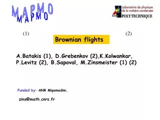
(1) (2) Brownian flights A.Batakis (1), D.Grebenkov (2),K.Kolwankar, P.Levitz (2), B.Sapoval, M.Zinsmeister (1) (2) Funded by: ANR Mipomodim, zins@math.cnrs.fr
The polymers that possess electrical charges (polyelectrolytes) are soluble in the water because of hydrogen bondings. The water molecules exhibit a dynamics made of adsorptions (due to hydrogen bondings) on the polymers followed by Brownian diffusions in the liquid.
The dynamics of the water molecules can be seen as an intermittent one: flights around the surface (« quick motion ») followed by a « slow » motion on the surface itself. In this talk we will ignore the adsorption steps. We are interested in the statistics of the flights , that is their duration and their length and wish to connect them to the geometry of the surface.
First passage statistics for and Brownian flights over a fractal nest: P.L et al; P.R.L. (May 2006)
Polymers and colloids in suspension exhibit rich and fractal geometry:
Main point: These statistics can be measured in experiences by using relaxometry methods in NMR (nuclear magnetic resonance).
I(t) NMR Relaxation L R1slow(f) a FTt(<I(0).I(t)>) A I(t) L L B0 time A R1Slow(f) A f NMR EXPERIMENTATION I(t+t)
Mathematical simulation of a flight: We consider a surface or a curve which is fractal up to a certain scale, typically a piecewise affine approximation of a self-affine curve or surface. We then choose at random an affine piece and consider a point in the complement of the surface nearby this piece. We then start a Brownian motion from this point stopped when it hits back the surface and consider the length and duration of this flight.
We have to precise the term « random »: If we consider only one flight there are two natural models: Uniform law: all points at a fixed vicinity of the surface have the same probability of being chosen as the starting point The point is chosen as the first hitting point on the surface of a Brownian motion started from a distinguished point :=the harmonic measure
In practise it is impossible to decide if it is the first flight. If m is a distribution on the boundary, the law of the hitting point at the end of the flight is a new distribution T(m) Is there an invariant distribution? If one starts the process with one of the 2 above mentionned distributions, does the law of the nth hitting point converge to an invariant distribution?
2) Experimenal results: If we want to perform experiments one problem immediately arises: The flights we consider are not first flights. One solution: to use molecules that are non-fractal and homogeneous
First Test: Probing a Flat Surface AFM Observations An negatively charged particle P.L et al Langmuir (2003)
EXPERIMENTS VERSUS ANALYTICAL MODEL FOR FLAT INTERFACES Laponite Glass at C= 4% w/w a=3/2 P.L. et al Europhysics letters, (2005), P.L. J. Phys: Condensed matter (2005)
Water NMR relaxation Almost Dilute suspension of Imogolite colloids
Magnetic Relaxation Dispersion of Lithium Ion in Solution of DNADNA from Calf Thymus(From B. Bryant et al, 2003) R1(s-1)
Brownian Exponants exponents: Influence of the surface roughness: Self similarity/ Self affinity(D. Grebenkov, K.M. Kolwankar, B. Sapoval, P. Levitz) 3D 2D
dsurface=1.25 POSSIBLE EXTENSION TO LOW MINKOWSKI DIMENSIONS: (1<dsurface<2 with dambiant=3)
4) A simple 2D model. We consider a simple 2D model for which we can rigorously derive the statistics of flights. In this model the topological structure of the level lines of the distance-to-the-curve function is trivial.
Case of the second flight: There is an invariant measure equivalent with harmonic measure
v U u General case: we want to compare the probability P(u,v,U) that a Brownian path started at u touches the red circle of center v and radius half the distance from v to the boundary of U before the boundary of U with its analogue P(v,u,U)
This last result is not true in d=2 without some extra condition. But we are going to assume this condition anyhow to hold in any dimension since we will need it for other purposes. In dimension d it is well-known that sets of co-dimension greater or equal to 2 are not seen by Brownian motion. For the problem to make sense it is thus necessary to assume that the boundary is uniformly « thick ». This condition is usually defined in terms of capacity. It is equivalent to the following condition:
Every open subset in the d-dimensional space can be partitionned (modulo boundaries) as a union of dyadic cubes such that: (Whitney decomposition) For all integers j we define Wj =the number of Whitney cubes of order j.
We now wish to relate the numbers Wj to numbers related to Minkowski dimension. For a compact set E and k>0 we define Nk as the number of (closed) dyadic cubes of order k that meet E.
This gives a rigourous justification of the results of the simulations in the case of the complement of a closed set of zero Lebesgue measure. For the complement of a curve in 2D in particular, it gives the result if we allow to start from both sides.
A pair (U,E) where U is a domain and E its boundary is said to be porous if for every x in E and r>0 (r<diam(E)) B(x,r) contains a ball of radius >cr also included in U. U
If the pair (U,E) is porous it is obvious that the numbers Wj and Nj are essentially the same. So if the domain is porous, have a « thick » boundary and a Minkowski dimension, then the power-law satisfied by the statistics of the flights is the expected one. Problem: the domain left to a SAW is not porous.
Self-Avoiding Walk, S.A.W. d=4/3
Theorem (Beffara, Rohde-Schramm): The dimension of the SLEk curve is 1+k/8. Theorem (Rohde-Schramm): The conformal mapping from UHP onto Ut is Holder continuous (we say that Ut is a Holder domain).