Geometric Index Structures for Multidimensional Data Management
250 likes | 359 Vues
Learn about practical geometric index structures for organizing multidimensional data efficiently. Topics include B-trees, stabbing query problems, and planar point locations. Explore hash-like indexes, tree-based indexes, and various query types.

Geometric Index Structures for Multidimensional Data Management
E N D
Presentation Transcript
Advanced Database Technology Anna Östlin Pagh and Rasmus Pagh IT University of Copenhagen Spring 2004 Geometric index structures April 15, 2004 Based on GUW Chapter 14.0-14.3, [Arge01] Sections 1, 2.1 (persistent B-trees), 3-4 (static versions only), 4.1, 9.
Today's lecture • Practical issues • Multidimensional data • Commonly used (heuristic) geometric index structures • Persistent B-trees • Stabbing query problem • Planar point location • The logarithmic method
Practical issues • Hand-ins • Course evaluation (9 out of 22) • Exercise sessions • Trial exam • The book • Scientific articles • Language • Extra exercise hour(s) in May/June • 4-week projects/thesis projects
Multidimensional data Geometric data is one, two, or three dimensional, but also all relational data can be seen as multidimensional data. • A relation with k attributes can be seen as a k-dimensional space. • A tuple can be seen as a point in the k-dimensional space. The coordinates for the point are the values for the attributes.
2-d range query Given the relation: Student(Name, age, enrolled_year) Find all students aged 30 to 40 who started to study before 2004. SELECT Name FROM Student WHERE age<=30 AND age>=40 and enrolled_year<2004;
Geometric index structures Hash-like indexes • Grid files (*) • Partitioned hash functions Tree-based indexes • Multiple-key indexes (*) • kd-trees (*) • Quad trees • R-trees (*) These indexes are heuristic, i.e., they are not (proved to be) worst case efficient.
Queries on geometric data • Partial match queries: look up all points matching one or more attributes. • Range queries: look up all points within a range for one or more attributes. • Nearest-neighbor: find the point nearest to a query point. • Where-am-I: given data in the form of geometric objects, find the objects that intersect the query point.
Grid files • Simple idea: • Split each dimension into intervals. • Put each point into a bucket corresponding to the intervals it lies in (Ex: GUW p. 677). • Overflow handling as in hash tables. • Supports partial match queries, range queries, and nearest neighbor queries (how?) • Bad case: All data along ”diagonal” - need many grid lines (in internal memory) to avoid large buckets. • Empty buckets? No problem, just hash!
Multiple-key index • Index for several attributes A, B, C,…: • Group index attributes as a tuple (A,B,C,…) • Order among tuples is lexicographic. • Make B-tree index according to this order. • (Note: Different exposition in GUW). • Efficiently supports partial match queries on a prefix of the attributes (corresponds to a range query). • Bad case: Partial match query on non-prefix, e.g., search for single value of last attribute.
kd-trees • Short for ”k-dimensional search tree”. • Change from ordinary search trees: • Each node is associated with a dimension. • An internal node partitions the points of its subtree along its dimension. • Dimensions rotate down the tree: 1,2,..,k,1,2,..k,1,2,… (Ex: GUW p. 691) • Supports partial match queries, range queries and nearest neighbor queries. • Bad case: Many points with same value in some dimension makes it impossible to split points well along this dimension.
R-trees • In a B-tree each interior node: • Corresponds to a 1-dimensional range. • ”Knows” the ranges of its children. • In an R-tree each interior node: • Corresponds to a k-dimensional rectangle. • ”Knows” the rectangles of its children. • Supports partial match queries, range queries and nearest neighbor queries,… • Flexible: All kinds of geometric objects (not just points) fit into rectangles. • Unspecified (and hard): Maintaining ”good” rectangles.
Persistent data structure • A persistent data structure supports queries on previous versions of the data structure. • A query specifies a time, e.g., “Was element x in the data structure at time t”? • Updates are only supported at current time, not in an earlier version. • Possible solution: Copy the data structure when it is updated. (Inefficient!) • Similar to the concept of temporal databases.
Persistent B-trees • One data structure representing all versions of the B-tree. • Elements have an existence interval: it exists from the time of insertion until time of deletion (or until now if it is still in the current version). • Nodes in the B-tree also have an existence interval. • Nodes and elements are alive in their existence intervals. • Invariant: A node contains (B) alive children in its existence interval. • Note: Nodes alive at time t make up a B-tree for elements alive at time t.
Searching and updates in persistent B-trees • Searching for x at time t can be done as usually in time O(logBN) in the tree consisting of nodes alive at time t. • Insertion of x is similar to normal insertion in a B-tree. If x should be inserted in leaf l, and l is full, then we have to maintain the new invariant. (Blackboard) • Deletion: The element is not deleted, but the time interval is updated. This may cause a violation of the invariant. (Read yourself)
Time and space for persistent B-trees • Construction: Insert elements one by one: N insertions take O(N logBN) I/Os. • In fact, construction can be done in O(N/B logM/B(N/B)) I/Os (not curriculum). • Space: O(N/B) blocks. • Note: N is the total number of elements, both alive and deleted elements.
Problem session Why are we talking about persistent B-trees in a lecture on geometric data? • How can we use a persistent B-tree to represent 2-d (geometric) data? • Given a set of points in 2-d, how can we perform a 3-sided, 2-d range query using the persistent B-tree?
Stabbing query problem • Data structure for a set of intervals (1-d). • Query: Report all intervals containing point q. • Static version. • Use the logarithmic method to get a dynamic data structure supporting insertions of intervals.
Stabbing query problem (cont.) • Use a persistent B-tree with intervals as elements and interval endpoints as times. • Sweep the intervals from left to right. • Insert an interval when the sweep line reaches it left endpoint. • Delete an interval when the sweep line reaches the right endpoint. • Construction time: O(N/B logM/B(N/B)) • Query: Report all elements alive at time q. O(logBN+T/B). (T=output size)
Planar point location • Given a planar subdivision with N vertices. • We want a data structure supporting: • Query: “Which region contains point q=(x,y)?” • Assume: Enough to find one segment of the region (the one straight above q).
Planar point location (cont.) • Idea: Use a persistent B-tree. • Segments are elements. • A segment exists in the time interval from left x-coordinate to right x-coordinate. • Search at time x (q=(x,y)). How do we find the right segment?
Problem session • Segments can not be ordered (in a given direction) in general. Why not? • We need an order of the segments to search in the B-tree. Which segments do we need to compare? • How can it be done?
Planar point location (cont.) • Search for ”segment” q=(x,y), in the persistent B-tree at time x. • A point can be compared to a segment. • Search time: O(logBN) I/Os. • Construction time: O(N logBN) I/Os. • Space: linear (O(N/B) blocks).
The logarithmic method • A general method to make many static data structures dynamic. • Internal memory version: • Partition the N elements into log N sets of size 20, 21, 22,…. • Build a static data structure for each set, denoted D0, D1, D2,…. • Every query has to query each of the sets. • Insertion: Find first empty Di. Build the structure Di with all elements in the Dj’s for j<i and the new element. • Note: 20+21+…+2i-1=2i-1 • Amortized cost: x is in at most log2N d.s.
The logarithmic method - external memory • logBN subsets • Di has size at most Bi • Query: Query all structures. • Insertion: Insert in smallest Di where |D1|+|D2|+…+|Di|<Bi. The new data structure for Di contains all elements in Dj, j≤i, and the new element. • Deletion: Mark elements deleted.
The logarithmic method - external memory (cont.) Analysis: • Assume a static structure with construction cost T(N) and query cost Q(N). • Query time: O(∑logBN Q(|Di|)). If Q(N)=O(logBN) then the query time is O(logB2N). • Amortized cost of insertion: • Note 1: Di may be smaller than Bi, and it is rebuilt more than once. Hence an element may be in Di during several rebuilds. • Note 2: At least Bi-1 new elements in Di each rebuild. • Note 3: An element never moves ”down”. • Assume T(N)=O(N/B logBN) then insertion costs O(logB2N) I/Os, amortized. (Blackboard.)

![Index Structures [13]](https://cdn2.slideserve.com/4887970/index-structures-13-dt.jpg)


![Index Structures [13]](https://cdn5.slideserve.com/9668621/index-structures-13-dt.jpg)
