Geometry IV
Geometry IV. Makoto Asai (SLAC) Geant4 Tutorial Course. Contents. Magnetic field Field integration and other types of field Geometry checking tools Geometry optimization Parallel geometry Moving objects. Defining a magnetic field. Magnetic field (1). Create your Magnetic field class

Geometry IV
E N D
Presentation Transcript
Geometry IV Makoto Asai (SLAC) Geant4 Tutorial Course
Contents • Magnetic field • Field integration and other types of field • Geometry checking tools • Geometry optimization • Parallel geometry • Moving objects Geometry IV - M.Asai (SLAC)
Magnetic field (1) • Create your Magnetic field class • Uniform field : • Use an object of the G4UniformMagField class G4MagneticField* magField = new G4UniformMagField(G4ThreeVector(1.*Tesla,0.,0.); • Non-uniform field : • Create your own concrete class derived from G4MagneticField and implement GetFieldValue method. void MyField::GetFieldValue( const double Point[4], double *field) const • Point[0..2] are position in global coordinate system, Point[3] is time • field[0..2] are returning magnetic field Geometry IV - M.Asai (SLAC)
Magnetic field (2) • Tell Geant4 to use your field • Find the global Field Manager G4FieldManager* globalFieldMgr = G4TransportationManager::GetTransportationManager() ->GetFieldManager(); • Set the field for this FieldManager, globalFieldMgr->SetDetectorField(magField); • and create a Chord Finder. globalFieldMgr->CreateChordFinder(magField); • /example/novice/N04/ExN04 is a good starting point Geometry IV - M.Asai (SLAC)
Global and local fields • One field manager is associated with the ‘world’ and it is set in G4TransportationManager • Other volumes can override this • An alternative field manager can be associated with any logical volume • The field must accept position in global coordinates and return field in global coordinates • By default this is propagated to all its daughter volumes G4FieldManager* localFieldMgr = new G4FieldManager(magField); logVolume->setFieldManager(localFieldMgr, true); where ‘true’ makes it push the field to all the volumes it contains, unless a daughter has its own field manager. • Customizing the field propagation classes • Choosing an appropriate stepper for your field • Setting precision parameters Geometry IV - M.Asai (SLAC)
Field integration • In order to propagate a particle inside a field (e.g. magnetic, electric or both), we solve the equation of motion of the particle in the field. • We use a Runge-Kutta method for the integration of the ordinary differential equations of motion. • Several Runge-Kutta ‘steppers’ are available. • In specific cases other solvers can also be used: • In a uniform field, using the analytical solution. • In a smooth but varying field, with RK+helix. • Using the method to calculate the track's motion in a field, Geant4 breaks up this curved path into linear chord segments. • We determine the chord segments so that they closely approximate the curved path. ‘Tracking’ Step Chords Real Trajectory Geometry IV - M.Asai (SLAC)
Tracking in field • We use the chords to interrogate the G4Navigator, to see whether the track has crossed a volume boundary. • One physics/tracking step can create several chords. • In some cases, one step consists of several helix turns. • User can set the accuracy of the volume intersection, • By setting a parameter called the “miss distance” • It is a measure of the error in whether the approximate track intersects a volume. • It is quite expensive in CPU performance to set too small “miss distance”. ‘Tracking’ Step Chords Real Trajectory "miss distance" Geometry IV - M.Asai (SLAC)
Tunable parameters • In addition to the “miss distance” there are two more parameters which the user can set in order to adjust the accuracy (and performance) of tracking in a field. • These parameters govern the accuracy of the intersection with a volume boundary and the accuracy of the integration of other steps. • The “delta intersection” parameter is the accuracy to which an intersection with a volume boundary is calculated. This parameter is especially important because it is used to limit a bias that our algorithm (for boundary crossing in a field) exhibits. The intersection point is always on the 'inside' of the curve. By setting a value for this parameter that is much smaller than some acceptable error, the user can limit the effect of this bias. realtrajectory Chord “delta intersection” boundary estimated intersection correct intersection Geometry IV - M.Asai (SLAC)
Tunable parameters • The “delta one step” parameter is the accuracy for the endpoint of 'ordinary' integration steps, those which do not intersect a volume boundary. This parameter is a limit on the estimation error of the endpoint of each physics step. • “delta intersection” and “delta one step” are strongly coupled. These values must be reasonably close to each other. • At most within one order of magnitude • These tunable parameters can be set by theChordFinder->SetDeltaChord( miss_distance ); theFieldManager->SetDeltaIntersection( delta_intersection ); theFieldManager->SetDeltaOneStep( delta_one_step ); • Further details are described in Section 4.3 (Electromagnetic Field) of the Application Developers Manual. Geometry IV - M.Asai (SLAC)
Customizing field integration • Runge-Kutta integration is used to compute the motion of a charged track in a general field. There are many general steppers from which to choose, of low and high order, and specialized steppers for pure magnetic fields. • By default, Geant4 uses the classical fourth-order Runge-Kutta stepper (G4ClassicalRK4), which is general purpose and robust. • If the field is known to have specific properties, lower or higher order steppers can be used to obtain the results of same quality using fewer computing cycles. • In particular, if the field is calculated from a field map, a lower order stepper is recommended. The less smooth the field is, the lower the order of the stepper that should be used. • The choice of lower order steppers includes the third order stepper G4SimpleHeum, the second order G4ImplicitEuler and G4SimpleRunge, and the first order G4ExplicitEuler. A first order stepper would be useful only for very rough fields. • For somewhat smooth fields (intermediate), the choice between second and third order steppers should be made by trial and error. Geometry IV - M.Asai (SLAC)
Customizing field integration • Trying a few different types of steppers for a particular field or application is suggested if maximum performance is a goal. • Specialized steppers for pure magnetic fields are also available. They take into account the fact that a local trajectory in a slowly varying field will not vary significantly from a helix. • Combining this in with a variation, the Runge-Kutta method can provide higher accuracy at lower computational cost when large steps are possible. • To change the stepper theChordFinder->GetIntegrationDriver() ->RenewStepperAndAdjust( newStepper ); • Further details are described in Section 4.3 (Electromagnetic Field) of the Application Developers Manual. Geometry IV - M.Asai (SLAC)
Other types of field • The user can create their own type of field, inheriting from G4VField, and an associated Equation of Motion class (inheriting from G4EqRhs) to simulate other types of fields. Field can be time-dependent. • For pure electric field, Geant4 has G4ElectricField and G4UniformElectricField classes. For combined electromagnetic field, Geant4 has G4ElectroMagneticField class. • Equation of Motion class for electromagnetic field is G4MagElectricField. G4ElectricField* fEMfield = new G4UniformElectricField( G4ThreeVector(0., 100000.*kilovolt/cm, 0.) ); G4EqMagElectricField* fEquation = new G4EqMagElectricField(fEMfield); G4MagIntegratorStepper* fStepper = new G4ClassicalRK4( fEquation, nvar ); G4FieldManager* fFieldMgr = G4TransportationManager::GetTransportationManager()-> GetFieldManager(); fFieldManager->SetDetectorField( fEMfield ); G4MagInt_Driver* fIntgrDriver = new G4MagInt_Driver(fMinStep, fStepper, fStepper->GetNumberOfVariables() ); G4ChordFinder* fChordFinder = new G4ChordFinder(fIntgrDriver); Geometry IV - M.Asai (SLAC)
Debugging geometries • An protruding volume is a contained daughter volume which actually protrudes from its mother volume. • Volumes are also often positioned in a same volume with the intent of not provoking intersections between themselves. When volumes in a common mother actually intersect themselves are defined as overlapping. • Geant4 does not allow for malformed geometries, neither protruding nor overlapping. • The behavior of navigation is unpredictable for such cases. • The problem of detecting overlaps between volumes is bounded by the complexity of the solid models description. • Utilities are provided for detecting wrong positioning • Optional checks at construction • Kernel run-time commands • Graphical tools (DAVID, OLAP) protruding overlapping Geometry IV - M.Asai (SLAC)
Optional checks at construction • Constructors of G4PVPlacement and G4PVParameterised have an optional argument “pSurfChk”. G4PVPlacement(G4RotationMatrix* pRot,const G4ThreeVector &tlate, G4LogicalVolume *pDaughterLogical, const G4String &pName, G4LogicalVolume *pMotherLogical, G4bool pMany, G4int pCopyNo, G4bool pSurfChk=false); • If this flag is true, overlap check is done at the construction. • Some number of points are randomly sampled on the surface of creating volume. • Each of these points are examined • If it is outside of the mother volume, or • If it is inside of already existing other volumes in the same mother volume. • This check requires lots of CPU time, but it is worth to try at least once when you implement your geometry of some complexity. Geometry IV - M.Asai (SLAC)
Debugging run-time commands • Built-in run-time commands to activate verification tests for the user geometry are defined • to start verification of geometry for overlapping regions based on a standard grid setup, limited to the first depth level geometry/test/run or geometry/test/grid_test • applies the grid test to all depth levels (may require lots of CPU time!) geometry/test/recursive_test • shoots lines according to a cylindrical pattern geometry/test/cylinder_test • to shoot a line along a specified direction and position geometry/test/line_test • to specify position for the line_test geometry/test/position • to specify direction for the line_test geometry/test/direction Geometry IV - M.Asai (SLAC)
Debugging run-time commands • Example layout: GeomTest: no daughter volume extending outside mother detected. GeomTest Error: Overlapping daughter volumes The volumes Tracker[0] and Overlap[0], both daughters of volume World[0], appear to overlap at the following points in global coordinates: (list truncated) length (cm) ----- start position (cm) ----- ----- end position (cm) ----- 240 -240 -145.5 -145.5 0 -145.5 -145.5 Which in the mother coordinate system are: length (cm) ----- start position (cm) ----- ----- end position (cm) ----- . . . Which in the coordinate system of Tracker[0] are: length (cm) ----- start position (cm) ----- ----- end position (cm) ----- . . . Which in the coordinate system of Overlap[0] are: length (cm) ----- start position (cm) ----- ----- end position (cm) ----- . . . Geometry IV - M.Asai (SLAC)
Debugging tools: DAVID • DAVID is a graphical debugging tool for detecting potential intersections of volumes • Accuracy of the graphical representation can be tuned to the exact geometrical description. • physical-volume surfaces are automatically decomposed into 3D polygons • intersections of the generated polygons are parsed. • If a polygon intersects with another one, the physical volumes associated to these polygons are highlighted in color (red is the default). • DAVID can be downloaded from the Web as external tool for Geant4 • http://geant4.kek.jp/~tanaka/ Geometry IV - M.Asai (SLAC)
Debugging tools: OLAP • Stand-alone batch application • Provided as extended example • Can be combined with a graphical environment and GUI Geometry IV - M.Asai (SLAC)
Material scanner • Measures material thickness in units of geometrical length, radiation length and interaction length. • It can be region sensitive, so that you can measure the thickness of one particular region. • /control/matScan • scan - Start material scanning. • theta - Define theta range. • phi - Define phi range. • singleMeasure - Measure thickness for one particular direction. • eyePosition - Define the eye position. • regionSensitive - Set region sensitivity. • region - Define region name to be scanned. Geometry IV - M.Asai (SLAC)
Smart voxelization • In case of Geant 3.21, the user had to carefully implement his/her geometry to maximize the performance of geometrical navigation. • While in Geant4, user’s geometry is automatically optimized to most suitable to the navigation. - "Voxelization" • For each mother volume, one-dimensional virtual division is performed. • Subdivisions (slices) containing same volumes are gathered into one. • Additional division again using second and/or third Cartesian axes, if needed. • "Smart voxels" are computed at initialisation time • When the detector geometry is closed • Does not require large memory or computing resources • At tracking time, searching is done in a hierarchy of virtual divisions Geometry IV - M.Asai (SLAC)
Detector description tuning • Some geometry topologies may require ‘special’ tuning for ideal and efficient optimisation • for example: a dense nucleus of volumes included in very large mother volume • Granularity of voxelisation can be explicitly set • MethodsSet/GetSmartless() from G4LogicalVolume • Critical regions for optimisation can be detected • Helper class G4SmartVoxelStatfor monitoring time spent in detector geometry optimisation • Automatically activated if /run/verbose greater than 1 Percent Memory Heads Nodes Pointers Total CPU Volume ------- ------ ----- ----- -------- --------- ----------- 91.70 1k 1 50 50 0.00 Calorimeter 8.30 0k 1 3 4 0.00 Layer Geometry IV - M.Asai (SLAC)
Visualising voxel structure • The computed voxel structure can be visualized with the final detector geometry • Helper class G4DrawVoxels • Visualize voxels given a logical volume G4DrawVoxels::DrawVoxels(const G4LogicalVolume*) • Allows setting of visualization attributes for voxels G4DrawVoxels::SetVoxelsVisAttributes(…) • useful for debugging purposes Geometry IV - M.Asai (SLAC)
Parallel navigation • In the previous versions, we have already had several ways of utilizing a concept of parallel world. But the usages are quite different to each other. • Ghost volume for shower parameterization assigned to G4GlobalFastSimulationManager • Readout geometry assigned to G4VSensitiveDetector • Importance field geometry for geometry importance biasing assigned to importance biasing process • Scoring geometry assigned to scoring process • We merge all of them into common parallel world scheme. • Readout geometry for sensitive detector will be kept for backward compatibility. • Other current “parallel world schemes” became obsolete. Geometry IV - M.Asai (SLAC)
Parallel navigation • Occasionally, it is not straightforward to define sensitivity, importance or envelope to be assigned to volumes in the mass geometry. • Typically a geometry built machinery by CAD, GDML, DICOM, etc. has this difficulty. • New parallel navigation functionality allows the user to define more than one worlds simultaneously. • New G4Transportation process sees all worlds simultaneously. • A step is limited not only by the boundary of the mass geometry but also by the boundaries of parallel geometries. • Materials, production thresholds and EM field are used only from the mass geometry. • In a parallel world, the user can define volumes in arbitrary manner with sensitivity, regions with shower parameterization, and/or importance field for biasing. • Volumes in different worlds may overlap. Geometry IV - M.Asai (SLAC)
Parallel navigation • G4VUserParrallelWorld is the new base class where the user implements a parallel world. • The world physical volume of the parallel world is provided by G4RunManager as a clone of the mass geometry. • All UserParallelWorlds must be registered to UserDetectorConstruction. • Each parallel world has its dedicated G4Navigator object, that is automatically assigned when it is constructed. • Though all worlds will be comprehensively taken care by G4Transportation process for their navigations, each parallel world must have its own process to achieve its purpose. • For example, in case the user defines a sensitive detector to a parallel world, a process dedicated to this world is responsible to invoke this detector. G4SteppingManager sees only the detectors in the mass geometry. The user has to have G4ParallelWorldProcess in his physics list. Geometry IV - M.Asai (SLAC)
exampleN07 • Mass geometry • sandwich of rectangular absorbers and scintilators • Parallel scoring geometry • Cylindrical layers Geometry IV - M.Asai (SLAC)
Defining a parallel world main() (exampleN07.cc) G4VUserDetectorConstruction* geom = new ExN07DetectorConstruction; G4VUserParallelWorld* parallelGeom = new ExN07ParallelWorld("ParallelWorld"); geom->RegisterParallelWorld(parallelGeom); runManager->SetUserInitialization(geom); • The name defined in the G4VUserParallelWorld constructor is used as the physical volume name of the parallel world, and must be used for G4ParallelWorldProcess (refer to next slide). void ExN07ParallelWorld::Construct() G4VPhysicalVolume* ghostWorld = GetWorld(); G4LogicalVolume* worldLogical = ghostWorld->GetLogicalVolume(); • The world physical volume of the parallel is provided as a clone of the world volume of the mass geometry. The user cannot create it. • You can fill contents regardless of the volumes in the mass geometry. • Logical volumes in a parallel world needs not to have a material. Geometry IV - M.Asai (SLAC)
G4ParallelWorldProcess void ExN07PhysicsList::ConstructProcess() { AddTransportation(); ConstructParallelScoring(); ConstructEM(); } void ExN07PhysicsList::ConstructParallelScoring() { G4ParallelWorldProcess* theParallelWorldProcess = newG4ParallelWorldProcess("ParaWorldProc"); theParallelWorldProcess->SetParallelWorld("ParallelWorld"); theParticleIterator->reset(); while( (*theParticleIterator)() ){ G4ProcessManager* pmanager = theParticleIterator->value()->GetProcessManager(); pmanager->AddProcess(theParallelWorldScoringProcess); if(theParallelWorldProcess->IsAtRestRequired(theParticleIterator->value()) { pmanager->SetProcessOrderingToLast(theParallelWorldScoringProcess, idxAtRest); } pmanager->SetProcessOrdering(theParallelWorldScoringProcess, idxAlongStep, 1); pmanager->SetProcessOrderingToLast(theParallelWorldScoringProcess, idxPostStep); } } G4ParallelWorldProcess must be defined after G4Transportation but prior to any EM processes. Name of the parallel world defined by G4VUserParallelWorld constructor AlongStep must be 1, while AtRest and PostStep must be last Geometry IV - M.Asai (SLAC)
Layered mass geometries in parallel world • Suppose you implement a wooden brick floating on the water. • Dig a hole in water… • Or, chop a brick into two and place them separately… Geometry IV - M.Asai (SLAC)
Layered mass geometries in parallel worlds • Parallel geometry may be stacked on top of mass geometry or other parallel world geometry, allowing a user to define more than one worlds with materials (and region/cuts). • Track will see the material of top-layer, if it is null, then one layer beneath. • Alternative way of implementing a complicated geometry • Rapid prototyping • Safer, more flexible and powerful extension of the concept of “many” in Geant3 Mass world Parallel world Geometry IV - M.Asai (SLAC)
Layered mass geometries in parallel worlds - continued • A parallel world may be associated only to some limited types of particles. • May define geometries of different levels of detail for different particle types • Example for sampling calorimeter: the mass world defines only the crude geometry with averaged material, while a parallel world with all the detailed geometry. Real materials in detailed parallel world geometry are associated with all particle types except e+, e- and gamma. • e+, e- and gamma do not see volume boundaries defined in the parallel world, i.e. their steps won’t be limited • Shower parameterization such as GFLASH may have its own geometry Geometry seen by e+, e-, g Geometry seen by other particles Geometry IV - M.Asai (SLAC)
G4ParallelWorldProcess void ExN07PhysicsList::ConstructParallelScoring() { G4ParallelWorldProcess* theParallelWorldProcess = new G4ParallelWorldProcess("ParaWorldProc"); theParallelWorldProcess->SetParallelWorld("ParallelWorld"); theParallelWorldProcess->SetLayeredMaterialFlag(); theParticleIterator->reset(); while( (*theParticleIterator)() ){ G4ProcessManager* pmanager = theParticleIterator->value()->GetProcessManager(); pmanager->AddProcess(theParallelWorldScoringProcess); if(theParallelWorldProcess->IsAtRestRequired(theParticleIterator->value()) { pmanager->SetProcessOrderingToLast(theParallelWorldScoringProcess, idxAtRest); } pmanager->SetProcessOrdering(theParallelWorldScoringProcess, idxAlongStep, 1); pmanager->SetProcessOrderingToLast(theParallelWorldScoringProcess, idxPostStep); } } Switch of making G4ParallelWorldProcess check materials in parallel world Geometry IV - M.Asai (SLAC)
4D RT Treatment Plan Source: Lei Xing, Stanford University …… + + + Ion chamber Lower Jaws Upper Jaws MLC Geometry IV - M.Asai (SLAC)
Moving objects • In some applications, it is essential to simulate the movement of some volumes. • E.g. particle therapy simulation • Geant4 can deal with moving volume • In case speed of the moving volume is slow enough compared to speed of elementary particles, so that you can assume the position of moving volume is still within one event. • Two tips to simulate moving objects : • Use parameterized volume to represent the moving volume. • Do not optimize (voxelize) the mother volume of the moving volume(s). Geometry IV - M.Asai (SLAC)
Moving objects - tip 1 • Use parameterized volume to represent the moving volume. • Use event number as a time stamp and calculate position/rotation of the volume as a function of event number. void MyMovingVolumeParameterisation::ComputeTransformation (const G4int copyNo, G4VPhysicalVolume *physVol) const { static G4RotationMatrix rMat; G4int eID = 0; const G4Event* evt = G4RunManager::GetRunManager()->GetCurrentEvent(); if(evt) eID = evt->GetEventID(); G4double t = 0.1*s*eID; G4double r = rotSpeed*t; G4double z = velocity*t+orig; while(z>0.*m) {z-=8.*m;} rMat.set(CLHEP::HepRotationX(-r)); physVol->SetTranslation(G4ThreeVector(0.,0.,z)); physVol->SetRotation(&rMat0); } Null pointer must be protected.This method is also invoked while geometry is being closed atthe beginning of run, i.e. event loop has not yet began. Here, event number is convertedto time.(0.1 sec/event) You are responsible not to make the moving volume get out of(protrude from) the mother volume. Position and rotationare set as the functionof event number. Geometry IV - M.Asai (SLAC)
Moving objects - tip 2 • Do not optimize (voxelize) the mother volume of the moving volume(s). • If moving volume gets out of the original optimized voxel, the navigator gets lost. motherLogical -> SetSmartless( number_of_daughters); • With this method invocation, the one-and-only optimized voxel has all daughter volumes. • For the best performance, use hierarchal geometry so that each mother volume has least number of daughters. Geometry IV - M.Asai (SLAC)