Acoustic peaks in CMBR and Relativistic Heavy Ion Collisions : Discussions

1. Acoustic peaks in CMBR and Relativistic Heavy Ion Collisions : Discussions Ajit M. Srivastava Institute of Physics Bhubaneswar

2. Recall: Important Points of our model QGP phase a transient stage, lasts for ~ 10-22 sec. Finally only hadrons detected carrying information of the system at freezeout stages (chemical/ thermal freezeout). This is quite like CMBR which carries the information at The surface of last scattering in the universe. Just like for CMBR, one has to deduce information about The earlier stages from this information contained in hadrons Coming from the freezeout surface. We have argued that this apparent correspondence with CMBR is in fact much deeper There are strong similarities in the nature of density fluctuations in the two cases (with the obvious difference of the absence of gravity effects for relativistic heavy-ion collision experiments).

3. Consider: Central collisions ; Same considerations apply for non-central collisions also It has been noticed that even in central collisions, due to initial state fluctuations, one can get non-zero anisotropies in particle distribution (and hence in final particle momenta) in a given event. These will be typically much smaller in comparison to the non-central collisions, and will average out to zero when large number of events are included. For a given central event azimuthal distribution of particles and energy density in general anisotropic: due to fluctuations of nucleon coordinates also due to localized nature of parton production during initial nucleon collisions.

4. Contour plot of initial (t = 1 fm) transverse energy density for Au-Au collision at 200 GeV/A center of mass energy, obtained using HIJING Azimuthal anisotropy of produced partons is manifest in this plot. Thus: reasonable to expect that the equilibrated matter will also have azimuthal anisotropies (as well as radial fluctuations) of similar level

5. The process of equilibration will lead to some level of smoothening. However, thermalization happens quickly (for RHIC, within 1 fm) No homogenization can be expected to occur beyond length scales larger than this. Thus, inhomogeneities, especially anisotropies with wavelengths larger than the thermalization scale should be necessarily present at the thermalization stage when the hydrodynamic description is expected to become applicable.This brings us to the most important correspondence between the universe and relativistic heavy-ion collisions: It is the presence of fluctuations with superhorizon wavelengths. Recall: In the universe, density fluctuations with wavelengths of superhorizon scale have their origin in the inflationary period.

6. First note: Relevant experimental observables: For the case of the universe, density fluctuations are accessible through the CMBR anisotropies which capture imprints of all the fluctuations present at the decoupling stage: For RHICE: the experimentally accessible data is particle momenta which are finally detected. Initial stage spatial anisotropies are accessible only as long as they leave any imprints on the momentum distributions (as for the elliptic flow) which survives until the freezeout stage. So: Fourier Analyze transverse momentum anisotropy of final particles (say, in a central rapidity bin) in terms of flow coefficients with n varying from 1 to large value ~30,40

7. The most important lesson for RHICE from CMBR analysis CMBR temperature anisotropies analyzed using Spherical Harmonics Now: Average values of these expansions coefficients are zero due to overall isotropy of the universe However: their standard deviations are non-zero and contain crucial information. Lesson : Apply same technique for RHICE also

9. For central events average values of flow coefficients will be zero (same is true even for non-central events if a laboratory fixed coordinate system is used). Following CMBR analysis, we propose to calculate Root-Mean-Square values of these flow coefficients using a lab fixed coordinate system: These values may be generally non-zero for even very large n and will carry important information Important: No need for the identification of any event plane So: Analysis much simpler. Straightforward Fourier series expansion of particle momenta

10. Acoustic peaks in CMBR anisotropy power spectrum (Resulting from coherence and acoustic oscilations of density fluctuations). Solid curve: Prediction from inflation Proposal for RHICE: Plot of for large values of n will give important information about initial density fluctuations. It may also reveal non-trivial structure like for CMBR, as we argue:

11. Inflationary Density Fluctuations: We know: Quantum fluctuations of sub-horizon scale are stretched out to superhorizon scales during the inflationary period. During subsequent evolution, after the end of the inflation,fluctuations of sequentially increasing wavelengths keep entering the horizon. The largest ones to enter the horizon, and grow, at the stage of decoupling of matter and radiation lead to the first peak in CMBR anisotropy power spectrum. We have seen that superhorizon fluctuations should be present in RHICE at the initial equilibration stage itself. Note: sound horizon, Hs = cs t , where cs is the sound speed, is smaller than 1 fm at t = 1 fm. With the nucleon size being about 1.6 fm, the equilibrated matter will necessarily have density inhomogeneities with superhorizon wavelengths at the equilibration stage.

12. We have argued that in RHICE also, coherence and acoustic oscillations may be present for flow anisotropies. Coherence resulting from the fact that the transverse velocities are zero to begin with. Acoustic oscillations seem natural, for small wavelengths: Due to unequal initial pressures in the two directions f1 and f2 momentum anisotropy will rapidly build up in these two directions in relatively short time. Expect: Spatial anisotropy should reverse sign in time of order l/(2cs)~ 2 fm (radial expansion may still not be dominant).

13. Now: super-horizon fluctuations: Recall: For CMBR, the importance of horizon entering is for the growth of fluctuations due to gravity. This leads to increase in the amplitude of density fluctuations, with subsequent oscillatory evolution, leaving the imprints of these important features in terms of acoustic peaks. For RHICE, there is a similar (though not the same, due to absence of gravity here) importance of horizon entering. We have argued that flow anisotropies for superhorizon fluctuations in RHICE should be suppressed by a factor where Hsfr is the sound horizon at the freezeout time tfr Note: Scaling of V_2 with c_s(t - t_0) is known (Bhalerao et al: PLB 627, 49 (2005)) Our model implies that similar scaling (by above factor) should apply to all superhorizon modes

14. Suppression of superhorizon anisotropies: Interface Sound horizon at freezeout When l >> Hsfr , then by the freezeout time full reversal of spatial anisotropy is not possible:The relevant amplitude for oscillation is only a factor of order Hsfr /(l /2) of the full amplitude.

15. We incorporate the above analysis in the estimates of spatial anisotropies for RHICE using HIJING event generator We calculate initial anisotropies in the fluctuations in the spatial extent R(f) (using initial parton distribution from HIJING) R(f) represents the energy density weighted average of the transverse radial coordinate in the angular bin at azimuthal coordinate f. We calculate the Fourier coefficients Fn of the anisotropies in where R is the average of R(f). Note: We represent fluctuations essentially in terms of fluctuations in the boundary of the initial region. May be fine for estimating flow anisotropies, especially in view of thermalization processes operative within the plasma region

16. For elliptic flow we know: Momentum anisotropy v2 ~ 0.2 spatial anisotropy e. For simplicity, we use same proportionality constant for all Fourier coefficients: Note: This does not affect any peak structures Important: In contrast to the conventional discussions of the elliptic flow, we do not try to determine any special reaction plane on event-by-event basis. A fixed coordinate system is used for calculating azimuthal anisotropies. Thus: This is why, as we will see, averages of Fn (and hence of vn) will vanish when large number of events are includedin the analysis. However, the root mean square values of Fn , and hence of vn , will be non-zero in general and will contain non-trivial information.

17. Results: HIJING parton distribution Errors less than ~ 2% uniform distribution of partons Include superhorizon suppression Include oscillatory factor also

18. From HIJING final particle momenta. HIJING Parton distribution Uniform distribution of partons with momentum cut-off no momentum cut-off

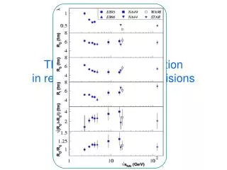
19. Paul Sorensen “Searching for Superhorizon Fluctuations in Heavy-Ion Collisions”, nucl-ex/0808.0503 Left panel: p_T autocorrelations derived from the <p_T> fluctuation scale dependence in Au+Au collisions at sqrt{s_NN} = 200 GeV. Sinusoidal modulations associated with v_2 have been subtracted. Right panel: p_T autocorrelations plotted in cylindrical coordinates. The positive near-side peak is subtracted revealing a valley.

20. Paul Sorensen, nucl-ex/0808.0503 The power spectrum from p_T fluctuations in heavy-ion collisions. C_l are calculated at midrapidity with theta=0

21. One important difference in favor of RHICE: For CMBR, for each l, only 2l+1 independent measurements are available, as there is only one CMBR sky to observe. This limits accuracy by the so called cosmic variance. In contrast, for RHICE: Each nucleus-nucleus collision (with same parameters like collision energy, centrality etc.) provides a new sample event (in some sense like another universe).Therefore with large number of events, it should be possible to resolve any signal present in these events as discussed here.

22. Plots of may reveal important information: • The overall shape of these plots should contain non-trivial information about the early stages of the system and its evolution. • For CMBR, anisotropy power spectrum plots reveal crucial • information about detailed nature of initial density fluctuations • (e.g. non-Gaussianity effects), So: Calculate 3-pt. functions etc. • Here, for RHICE also, these plots will directly relate to distribution • of density fluctuations of the initial produced matter • Important to note: This is true irrespective of the validity of the • physics of coherence and acoustic oscillations of our model. • This only follows from applying the very successful tools of • analysis of CMBR anisotropy power spectrum for the case RHICE

23. If any of the peaks shown in the plots are observed: 2) The first peak contains information about the freezeout stage. Being directly related to the sound horizon it contains information about the equation of state at that stage (just like the first peak of CMBR). We have checked, using HIJING, that the peak shifts to higher n for larger center of mass energies, and for heavier nuclei. Increasing speed of sound shifts the peak to smaller n as sound horizon becomes larger Effects of changing initial time of equilibration t_0 are nontrivial: increasing t_0 lowers value of n where plot flattens: implying changeover in nature of fluctuations happening at large scales

24. Like for CMBR, oscillatory peaks here should contain information about dissipative effects and coupling of different species with each other (by plotting flow coefficients of different particles). • We plot vn up to n = 30, which corresponds to wavelength of fluctuation of order 1 fm. Fluctuations with wavelengthssmaller than 1 fm cannot be treated within hydrodynamical framework. A changeover in the plot of vn for large n will indicate applicable regime of hydrodynamics. • 5) One important factor which can affect the shapes of these curves, especially the peaks, is the nature and presence of the quark-hadron transition. Clearly the duration of any mixed phase directly affects the freezeout time and hence the location of the first peak. • More importantly, any softening of the equation of state near the transition may affect locations of any successive peaks and their relative heights

25. Possibility of checking aspects of Inflationary physics in Lab? If one does see even the first peak for RHICE then one very important issue relevant for CMBR can be studied with controlled experiments. It is the issue of horizon entering. For example, by changing the nuclear size and/or collision energy, one can arrange the situation when first peak occurs at different values of n. Theoretical understanding of horizon entering of superhorizon fluctuations can be studied experimentally.

26. Full Hydrodynamical simulations can check these possibilities, we plan to do that. Meanwhile: check the evolution of (complex scalar) field with non-trivial boundaries. (Polyakov loop order parameter) Transverse expansion (radial flow) is visible below

27. Evolve field with initial configuration as shown below: Any surface waves (Edge states)? Expect similar behavior as for fluid expansion: Check for any oscillations. For QGP, hydrodynamical evolution simulates plasma. What about Polyakov loop condensate background ?

29. Quark-Hadron phase transition: Spontaneous breaking of Z(3) symmetry in the QGP phase For the confinement-deconfinement phase transition in a SU(N) gauge theory, the Polyakov Loop Order Parameter is defined as: Here, P denotes path ordering, g is the coupling, b = 1/ T, with T being the temperature, A0 (x,t)is the time component of the vector potential at spatial position x and Euclidean time t. Under a global Z(N) transformation, l(x) transforms as:

30. The expectation value of the Polyakov loop l0 is related to the Free energy F of a test quark l 0 ~ exp(-F/ T) l0 is non-zero in the QGP phase corresponding to finite energy of quark, and is zero in the confining phase. Thus, it provides an order parameter for the QCD transition, (with N = 3) As l0 transforms non-trivially under the Z(3) symmetry, its non-zero value breaks the Z(3) symmetry spontaneously in the QGP phase. The symmetry is restored in the Confining phase. Thus, there are Z(3) domain walls in the QGP phase Quarks lead to explicit breaking of Z(3) symmetry : Domain walls move away from the true vacuum

31. Let us first discuss the properties of these walls, and a new string like structure in the QGP phase. For numerical estimates, we use the following Lagrangian for l(x), proposed by Pisarski (no explicit symmetry breaking): Here, V(l) is the effective potential. Values of various parameters are fixed by making correspondence with Lattice results: b = 2.0, c = 0.6061 x 47.5/16, a(x) = (1-1.11/x)(1+0.265/x)2 (1+0.300/x)3 – 0.487 where, x = T/ Tc The value of Tc used is ~ 182 MeV. With suitable re-scaling, Note: b term gives cos 3q , leading to Z(3) vacuum structure

32. Plot of V(l) in units of TC4 for T = 185 MeV, l = |l|exp(iq) q = 0 |l| = l0 Note: relative heights of barriers

33. Compare : Axionic wall/string case Polyakov loop case