
Probit Regression
E N D
Presentation Transcript
Probit Regression Psych 818 - DeShon
Dichotomous Response • Probit regression is based on a different approach to the dichotomous response process • Assume that the right model is: • Y = bo + b1(X) + e • where e is a normally distributed error and Y is a continuous outcome • Y is latent and instead we observe a dichotomous response • Views dichotomous response as a coarse measurement issue
Dichotomous Responses • Observe Y=1; if Y > c • Observe Y=0; if Y < c • Use the normal distribution to determine the probability of a 1
Probit Model • The cumulative distribution function (cdf) is the integral of the pdf from −∞ to a point of interest • This gives the probability of obtaining a value less than (or equal to) X. • For the normal this is
Probit vs. Logit • logit = 1.7 probit • x <- seq(-5,5,.01) • x2 <- 1.7*x • # Adjust for different Logit scale • Px <- pnorm(x) • Lx <- 1/(1+exp(-x)) • Lxs <- 1/(1+exp(-x2)) • plot()
Analysis Example • GRE and grad school admissions • 400 students with GRE scores and admission status
Analysis Example • Logit Model • lr <- glm(ADMIT~GRE, family=binomial, data=df) • exp(lr$coefficients) • But GRE scores increment by 10, not 1 so.. • 1.0035886^10=1.036471 • 1 unit change in GRE increases odds of admissions by a factor of 1.03 Coefficients: (Intercept) GRE -2.901344 0.003582 (Intercept) GRE 0.0549493 1.0035886
Analysis Example • Logit model • Can use predicted probabilities to interpret the results • newdata1<-data.frame(GRE<-seq(220,800,10)) • newdata1$prob<-predict(lr,newdata=newdata1,type="response")
Analysis Example • Probit Model • pt<- glm(ADMIT ~ GRE, family=binomial(link="probit"), data=df) • Notice that the coefficients in the probit model are roughly 1.7 times the coefficients in the logit model Coefficients: (Intercept) GRE -1.768186 0.002175
Probit Results • Can be hard to interpret the coefficients from a probit model so predicted probabilities are commonly computed • newdata1$probpr <-predict(pr,newdata=newdata1,type="response")