Discrete Mathematical Structures
Discrete Mathematical Structures. 离散数学结构. Bernard Kolman Robert C. Busby Sharon Cutler Ross. 《 离散数学 》 教学组. Chapter 7 Trees. 7.1 Trees 7.2 Labeled Trees 7.3 Tree Searching 7.4 Undirected Trees 7.5 Minimal Spanning Trees. 7.1 Trees.


Discrete Mathematical Structures
E N D
Presentation Transcript
Discrete MathematicalStructures 离散数学结构 Bernard Kolman Robert C. Busby Sharon Cutler Ross 《离散数学》教学组
中山大学软件学院 Chapter 7 Trees 7.1 Trees 7.2 Labeled Trees 7.3 Tree Searching 7.4 Undirected Trees 7.5 Minimal Spanning Trees
中山大学软件学院 7.1 Trees Let A be a set, and let T be a relation on A. If there is a vertex v0 in A with the property that there exists a unique path in T from v0 to every other vertex in A, but no path from v0 to v0, then we say that T is a tree. The vertex v0, described in the definition of a tree, is unique. It is often called the root of the tree T, and T is then referred to as a rooted tree. We write (T, v0) to denote a rooted tree T with root v0. If (T, v0) is a rooted tree on the set A, an element v of A will often be referred to as a vertex in T.
中山大学软件学院 7.1 Trees Theorem 1 Let (T, v0) be a rooted tree. Then (a) There are no cycles in T. (b) v0 is the only root of T. (c) Each vertex in T, other than v0, has in-degree one, and v0 has in-degree zero. Proof (a) Suppose that there is a cycle q in T, beginning and ending at vertex v. By definition of a tree, we know that vv0, and there must be a path p from v0 to v. Then q◦p is a path from v0 to v that is different from p, and this contradicts the definition of a tree. (b) If v0 is another root of T, it is easy to get a contradiction.
中山大学软件学院 7.1 Trees (c) Let w1 be a vertex in T other than v0. Then there is a unique path v0, … , vk, w1 from v0 to w1 in T. So w1 has in-degree at least one. If the in-degree of w1 is more than one, there must be distinct vertices w2 and w3 such that (w2, w1) and (w3, w1) are both in T. If w2v0 and w2v0, there are paths p2 from v0 to w2 and p3 from v0 to w3, by definition. Then (w2, w1)◦p2 and (w3, w1)◦p3 are two different paths from v0 to w1, and this contradicts the definition of a tree with root v0. If w2=v0 or w2=v0, we leave it as an exercise to show that v0 has in-degree zero.
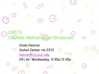
v0 v1 v3 v2 v0 v1 v2 v3 v4 v5 v6 v7 v8 v9 中山大学软件学院 7.1 Trees The digraph of a tree. The root v0 is said to be at level 0. The terminal vertices of the edges beginning at v0 are called the level 1 vertices. The terminal vertices of the edgesleaving a vertex at level 1 are calledthe level 2 vertices. The vertices at level 3, level 4,… are similarly defined. Level 0 Level 1 Level 0 Level 1 Level 2
中山大学软件学院 7.1 Trees The root v0 is called the parent of the level 1 vertices, and the level 1 vertices are called the offspring of v0. parent The parent-offspring relationship holds for the other vertices at every consecutive pair of levels. The offspring of any one vertex are called sibling (兄弟). The largest level number of a tree is called the height of the tree. The vertices of the tree that have no offspring are called the leaves of the tree. In the digraph of a tree, we assume some ordering of the offspring of each vertex by arranging them from left to right. Such a tree will be called an ordered tree. Height offspring sibling leaf
中山大学软件学院 7.1 Trees The following relational properties of trees are easily verified. Theorem 2 Let (T, v0) be a rooted tree on a set A. Then (a) T is irreflexive. (b) T is asymmetric. (c) If (a, b)T and (b, c)T, then (a, c)T, a, b, cA.
中山大学软件学院 7.1 Trees Ex. Let A be the set consisting of a given woman v0 and all of her female descendants. We now define the following relation T on A: v1Tv2iffv1 is the mother of v2. The relation T on A is a rooted tree with root v0. Ex. Let A={v1, v2, …, v10} and let T={(v2,v3), (v2,v1), (v4,v5), (v4,v6), (v5,v8),(v6,v7), (v4,v2), (v7,v9), (v7,v10)}. Show that T is a rooted tree andidentify the root. v4 v6 v2 v5 v7 v1 v3 v8 v9 v10 Figure 7.2
中山大学软件学院 7.1 Trees Let T be a tree and let n be a positive integer. If every vertex of T has at most n offspring,we say that T is an n-tree. If all vertices of T, other than the leaves,have exactly n offspring, we say that T is a complete n-tree. In particular, a 2-tree is often called abinary tree (二叉树), and a complete2-tree is often called a complete binarytree (完全二叉树). … n offspring complete binary tree
中山大学软件学院 7.1 Trees Let (T, v0) be a rooted tree on the set A, and let v be a vertex of T. Let B be the set consisting of v and all its descendants, B⊆A. Let T(v) be the restriction of the relation T to B, that is, T∩(BB). We will say that T(v) is the subtreeof T beginning at v.
中山大学软件学院 7.1 Trees Theorem 3 If (T, v0) is a rooted tree and vT, then T(v) is also a rooted tree with root v. Proof By definition of T(v), there is a path from v to every other vertex in T(v). If there is a vertex w in T(v) such that there are two distinct paths q and q from v to w, and let p be the path in T from v0 to v, then q◦p and q◦p would be two distinct paths in T from v0 to w. This contradicts that T is a tree with root v0. Also, if q is a cycle at v in T(v), then q is also a cycle in T. This contradicts Theorem 1(a), Thus, q cannot exist. It follows that T(v) is a tree with root v.
v4 v6 v2 v5 v6 v2 v5 v7 v1 v3 v8 v7 v1 v3 v8 v9 v10 v9 v10 中山大学软件学院 7.1 Trees Ex. Consider the tree T of Example 2.This tree has root v4 and shown inFigure 7.2. Draw the subtrees T(v5), T(v2), and T(v6) of T. Solution T(v6) T(v2) T(v5)
+ − − − + 3 2 x x 2 3 x 中山大学软件学院 7.2 Labeled Trees We will represent the vertices simply as dots and show the label of each vertex next to the dot representing that vertex. Ex. Use the labeled tree to represent the algebraic expression (3−(2x))+((x−2)−(3+x)).
+ − + 3 − 4 7 1 x + y x 7 y 2 中山大学软件学院 7.2 Labeled Trees Ex. Draw the labeled tree of the algebraic expression ((3(1−x))((4+(7−(y+2)))(7+(xy))))
中山大学软件学院 7.2 Labeled Trees Positional n-tree (按位n-树) Let (T, v0) be an n-tree. Each vertex in T has at most n offspring. We imagine that each vertex potentially has exactly n offspring, which would be ordered from 1 to n, but that some of the offspring in the sequence may be missing.
L R 2 3 L R R 3 1 2 1 L L L R 3 3 1 2 3 R R L R 1 2 3 L L R 中山大学软件学院 7.2 Labeled Trees Ex. One positional 3-tree. Ex. One positional binary tree (按位二元树).
中山大学软件学院 7.2 Labeled Trees Huffman code tree The simple ASCII code for the letters of the English alphabet represents each letter by a string of 0’s and 1’s of length 7. A Huffman code also uses strings of 0’s and 1’s, but the strings are of variable length. The more frequently used letters are assigned shorter strings. In this way messages may be significantly shorter than with ASCII code. A labeled positional binary tree is an efficient way to represent a Huffman code.
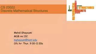
E A S R C 中山大学软件学院 7.2 Labeled Trees The string assigned to a letter gives a path from the root to the leaf labeled with that letter: (1). 0 the left (2). 1 the right Ex. Use the Huffman codetree in Figure 7.12 to decode thestring 0101100. Ex. If an error was made in transmittingstring 0101100 and string 0101110 is received,then the word read is EAR, not EASE. 0 1 0 1 0 1 0 10 110 0 E A S E 0 1 Figure 7.12 0 10 1110 0101100 0101110 E A R
中山大学软件学院 7.3 Tree Searching Performing appropriate tasks at a vertex will be called visiting the vertex. The process of visiting each vertex of a tree in some specific order will be called searching the tree or performing a tree search. In some texts, this process is called walking or traversing the tree. Let T be a binary tree with root v. If vL exists, the subtree T(vL) will be called the left subtree of T. If vR exists, the subtree T(vR) will be called the right subtree of T. 23
中山大学软件学院 7.3 Tree Searching Consider the following algorithm for searching a positional binary tree T with root v. PreOrder algorithm-先序遍历 (1). Visit v. (2). If vL exists, then apply this algorithm to (T(vL), vL). (3). If vR exists, then apply this algorithm to (T(vR), vR). Informally, the preorder search of a tree consists of the following three steps: (1). Visit the root. (2). Search the left subtree if it exists. (3). Search the right subtree if it exists.
A B H C E I K D F G J L 中山大学软件学院 7.3 Tree Searching Ex. T is the labeled, positional binary tree which digraph is shown in Figure 7.14. The root of this tree is the vertex A. Apply the preorder search algorithm to this tree. Solution Vertex Order: Finished A B C D E F G H I J K L
- + a b c d e 中山大学软件学院 7.3 Tree Searching Ex. Consider the parenthesized expression (a-b)(c+(de)). Figure 7.15 is the digraph of the labeled, positional binary tree representation of this expression. We apply the PreOrder to this tree, and get string -ab+cde. This is the prefix or Polish form (波兰式) of the given algebraic expression. a=6, b=4, c=5, d=2, e=2.
A B H C E I K D F G J L 中山大学软件学院 7.3 Tree Searching Consider the following informal algorithm of two other procedures for searching a positional binary tree T with root v. InOrder algorithm-中序遍历 (1). Search the left subtree (T(vL), vL) if it exists. (2). Visit the root v. (3). Search the right subtree (T(vR), vR) if it exists. Vertex Order: Finished D C B F E G A I J H K L
A B H C E I K D F G J L 中山大学软件学院 7.3 Tree Searching PostOrder algorithm-后序遍历 (1). Search the left subtree (T(vL), vL) if it exists. (2). Search the right subtree (T(vR), vR) if it exists. (3). Visit the root v. Vertex Order: Finished D C F G E B J I L K H A
1 2 4 3 5 6 7 8 9 10 11 12 13 中山大学软件学院 7.3 Tree Searching Ex. Figure 7.16(a) is the digraph of a labeled tree T. We draw a left edge from each vertex v to its first offspring (if v has offspring). We draw a right edge from each vertex v to its next sibling in the order given if v has a next sibling. 1 2 3 5 8 4 11 6 9 12 7 10 13
中山大学软件学院 7.4 Undirected Trees An Undirected tree T is simply the symmetric closure of a tree. The graph of an Undirected tree T will have a single line without arrows connecting vertices a and b when (a, b) and (b, a) belong to T. The set {a, b}, where (a, b) and (b, a) are in T, is called an undirected edge of T, vertex a and b are called adjacent vertices.
b a b d c c c g d a e d e f a b e f f g g 中山大学软件学院 7.4 Undirected Trees Ex. (a) is the graph of an undirected edge of T. (b) and (c) are digraphs of ordinary tree T1 and T2, which have T as symmetric closure. Relation T contains 12 pairs. An undirected tree can correspond to many directed trees. (a) (b) (c)
a f e b c d 中山大学软件学院 7.4 Undirected Trees Let R be a symmetric relation, and let p: v1, v2, …, vn be a path in R. p is simple if no two edges of p correspond to the same undirected edge. If p is a cycle (v1=vn), p is called a simple cycle. Ex. The graph of a symmetric relationis showed on right. The path a, b, c, e, d is simple. The path f, e, d, c, d, a is not simplesince {d,c} and {c,d} are same. d, a, b, d is a simple cycle. f, e, d, c, e, f is not a simple cycle.
中山大学软件学院 7.4 Undirected Trees A symmetric relation R is acyclic(无环的) if it is contains no simple cycles. Theorem 1 Let R be a symmetric relation on a set A. Then the following statements are equivalent. (1). R is an undirected tree. (2). R is connected and acyclic. Theorem 2 Let R be a symmetric relation on a set A. Then R is a undirected tree iff either of the following statements is true. (1). R is acyclic, and if any undirected edge is added to R, the new relation will not be acyclic. (2). R is connected, and if any undirected edge is removed from R, the new relation will not be connected. Theorem 3 A tree with n vertices has n-1 edges.
a a a b c c b c b d e e e d d f f a f b c e d f 中山大学软件学院 7.4 Undirected Trees Spanning Trees of Connected Relations If R is a symmetric, connected relation on a set A, a tree on A is a spanning tree for R if T is a tree with exactly the same vertices as R and which can be obtained from R by deleting some edges of R. Ex. (a) (b) (c) (d)
中山大学软件学院 7.4 Undirected Trees Spanning Trees of Connected Relations Ex. Repeat the graph of Figure 7.31(a). The result of successive removal of undirected edges in Figure 7.32(f). Remove edges: {a,b}, {a,c} {b,c} {c,e} {d,e} a b c d e f
中山大学软件学院 7.4 Undirected Trees Spanning Trees of Connected Relations The operation of Shrinking(收缩) edge between vi and vj: move two vertices together and merge two vertices into v. (v, vt)E (vi, vt)E or (vj, vt)E Ex. Show the operations of shrinking edges. (1). Shrink (v0, v1), merge v0 and v1 into v0 (2). Shrink (v0, v2), merge v0 and v2 into v0 v0 v0 v0 v1 v2 v5 v4 v6 v3 24
中山大学软件学院 7.4 Undirected Trees Spanning Trees of Connected Relations Suppose that vertices a and b of a relation R are merged into a new vertex a that replaces a and b to obtain the relation R. To determine the matrix of R, the process is following: (1). Let row i represent vi(vertex) and row j represent vj. Replace row i by the join of rows i and j. rowi rowi rowj (2). Replace column i by the join of columns i and j. coli coli colj (3). Restore the main diagonal to its original values in R. (4). Delete row j and column j.
v0 v1 v2 v5 v4 v6 v3 中山大学软件学院 7.4 Undirected Trees Spanning Trees of Connected Relations Ex. Figure 7.34 is the matrices for the corresponding symmetric relations whose graphs are given in Figure 7.33. v0v1v2v3v4v5v6 v0v2v3v4v5v6 v0 v1 v2 v3 v4 v5 v6 0 1 1 0 0 1 0 1 0 0 1 1 0 0 1 0 0 0 0 1 1 0 1 0 0 0 0 0 0 1 0 0 0 0 0 1 0 1 0 0 0 0 0 0 1 0 0 0 0 v0 v2 v3 v4 v5 v6 0 1 1 1 1 0 1 1 1 1 0 0 0 0 1 1 0 0 0 0 0 0 0 0 0 0 1 0 0 0 0 1 0 0 0 0 v0v3v4v5v6 v0 v3 v4 v5 v6 0 1 1 1 1 1 1 1 1 0 0 0 0 0 0 0 0 0 0 0 0 0 0 0 0
中山大学软件学院 7.4 Undirected Trees Spanning Trees of Connected Relations Prim’s algorithm is an algorithm for finding a spanning tree for a symmetric, connected relation R on the set A={v1, …, vn}. (1). Choose a vertex v1 of R and arrange the matrix of R so that the first row corresponds to v1. (2). Choose a vertex v2 of R such that (v1, v2)R, merge v1 and v2 into a vertex v1, representing {v1, v2} and replace v1 by v1. Compute the matrix of the result relation R. (3). Repeat (1) and (2) on R until the relation has one vertex. (4). Construct the spanning tree: when merging vi and vj, select the edge (vi, vj) in R.
中山大学软件学院 7.4 Undirected Trees Spanning Trees of Connected Relations Ex. Apply Prim’s algorithm to relation whose graph is shown inFigure 7.35. abcd a b c d 0 0 1 1 0 0 1 1 1 1 0 0 1 1 0 0 a a a a b abd a{a,c} a b d 0 1 1 1 0 1 1 1 0 ad a{a,b} c d a d 0 1 1 0 a a{a,d} a 0
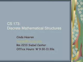
B H D 6 2 3 3 2 5 6 E C 2 A 3 5 4 4 G F 中山大学软件学院 7.5 Minimal Spanning Trees A weighted graph (加权图) is a graph for which each edge is labeled with a numerical value call its weight(权). We write a weighted graph as G=(V, E, W). The weight of an edge (vi, vj), written as w(vi, vj), is referred to as the distance between vertices vi and vj. Ex. w(A, B)=3 w(E, F)=4 w(vi, vj)= if (vi, vj)E. w(A, D)= w(B, E)=
V V1 中山大学软件学院 7.5 Minimal Spanning Trees Suppose that G=(V, E, W), V1V, A vertex u is a nearest neighbor of vertex v if w(u, v) = min{w(vi, v) | (vi, v)E} Vertex v has more than one nearest neighbor. The nearest neighbor vertex of A is C, The nearest neighbor vertices of F are E and G. A vertex v is a nearest neighbor of V1 in G if vjV1, w(v, vj) = min{ w(u, vi) | uV, viV1 } This vertex v may belong to V. v
B 2.6 C 2.7 2.1 4.2 A 2.4 2.9 E 3.6 2.2 3.3 3.4 I D 4.4 2.1 1.8 2.8 J H F 2.5 1.7 3.2 3.3 G 中山大学软件学院 7.5 Minimal Spanning Trees Ex. V={A, B, C, D, E, F, G, H, I, J}, V1={C, E, J}. Vertex D is a nearest neighbor V1 because w(D, E) is the least weight for all edges between V1 and V.
中山大学软件学院 7.5 Minimal Spanning Trees With applications of weighted graphs, it is necessary to find an undirected spanning tree for which the total weight of the edges in the tree is as small as possible. Such a spanning tree is called a minimal spanning tree. There are two algorithms (Prim and Kruskal)for producing a minimal spanning tree for a weighted graph.
中山大学软件学院 7.5 Minimal Spanning Trees PRIM’s Algorithm: Let R be a symmetric, connected relation with n vertices. (1). Choose a vertex v1 of R. Let V={v1} and E={}; (2). Choose a nearest neighbor vi of V that is adjacent to vj, vj V, and for which the edge (vi, vj) does not form a cycle with member of E. VV∪{vi}, EE∪{(vi, vj)} (3). Repeat Step 2 until |E|=n-1. (4). V contains all n vertices of R, and E contains the edges of a minimal spanning tree for R.
中山大学软件学院 7.5 Minimal Spanning Trees Prim’s Algorithm is an example of a greedy algorithm (贪心算法). At each step algorithm chooses what is “best” based on local conditions, rather than looking for global situation. Greedy algorithms do not always produce optimal solutions, but the solution of Prim’s algorithm is optimal.
中山大学软件学院 7.5 Minimal Spanning Trees Theorem 1. Prim’s algorithm produces a minimal spanning tree for the relation. Proof Let R have n vertices, let T be the spanning tree for R produced by Prim’s algorithm. Suppose that the edges of T, in the order in which they were selected, are e1, e2, …, en-1. For each i from 1 to n-1, we define Ti to be the tree with e1, e2, …, ei and T0={ }. Then T0 T1 … Tn-1=T. Now we prove that each Ti is contained in a minimal spanning tree for R.
中山大学软件学院 7.5 Minimal Spanning Trees Basic Step P(0): T0={ } is contained in every minimal spanning tree for R. Induction Step ……
B H D 6 2 3 3 2 5 6 E C 2 A 3 5 4 4 G F 中山大学软件学院 7.5 Minimal Spanning Trees Ex. Social Circle plans to pave some of the walking trails to make them bicycle paths as well. Assuming that construction costs are the same on all parts of the system, use Prim’s algorithm to find a plan for the town’s paving. B H D 2 3 2 E C 2 Solution We choose A as the first vertex. A 3 5 4 G F
B 2.6 C 2.7 A 2.1 4.2 2.4 2.9 E 3.6 2.2 3.3 3.4 I D 4.4 2.1 1.8 2.8 J H F 2.5 1.7 3.2 3.3 G 中山大学软件学院 7.5 Minimal Spanning Trees Ex. A minimal spanning tree for the communication network may be found by using Prim’s algorithm beginning at any vertex. We beginning at I for minimal spanning tree. The total cost of upgrading these links would be $20200000. B 2.6 C A 2.1 2.4 E 2.2 I D 2.1 1.8 2.8 J H F 2.5 1.7 G
4 A B 3 3 5 D 2 C 中山大学软件学院 7.5 Minimal Spanning Trees Now we expressed the weighted graph with matrix. The key to the modification is to consider an entry in the matrix as representing not only the existence of an edge, but also the weight of the edge. We construct a matrix containing the weights of edges, with a 0 to show there is no edge between a pair of vertices. Figure 7.55 shows a connected weighted graph and the associated matrix of weights. A B C D A B C D 0 4 3 0 4 0 5 3 3 5 0 2 0 3 2 0 Figure 7.55
中山大学软件学院 7.5 Minimal Spanning Trees PRIM’s Algorithm (Matrix Version) Let R be a symmetric, connected relation with n vertices and M be the associated matrix of weights. (1) Choose the smallest entry in M, say mij. Let vi and vj be the vertices that are represented by row i and column j. (2) Merge vi with vj as follows: Replace row i with (1kn) mikmjk=0 mjkmik=0 min(mik,mjk) mik0, mjk0 0 mik=mjk=0 mik =