More about Polynomials
10. More about Polynomials. Case Study. 10 .1 Polynomials and Their Operations. 10 .2 Division of Polynomials. 10 .3 Remainder Theorem. 10 . 4 Factor Theorem and Its Applications. 10 . 5 The G.C.D. and the L.C.M. of Polynomials. 10 . 6 Algebraic Fractions. Chapter Summary.

More about Polynomials
E N D
Presentation Transcript
10 More about Polynomials Case Study 10.1Polynomials and Their Operations 10.2 Division of Polynomials 10.3 Remainder Theorem 10.4 Factor Theorem and Its Applications 10.5The G.C.D. and the L.C.M. of Polynomials 10.6Algebraic Fractions Chapter Summary
If the volume of each pillar is 22 500pcm2, how can we find the radius of the spherical part? We need to use a polynomial to represent the volume of the pillar. By solving the equation obtained, we can find the radius. Case Study Since we know the total volume of the pillar, we can then set up an equation containing r, where r is the radius of the sphere. However, equations involving volumes in terms of radii are usually of degree 3, which are not easy to solve. We are going to learn a method to solve such kind of equations.
The degree of the polynomial is the same as the degree of the highest degree term. We usually write the polynomials in descending order of the degrees of terms. 10.1 Polynomials and Their Operations A. Polynomials in One Variable In junior forms, we discovered that an algebraic expression, like x3 2x2 3x 5, is an example of polynomials in one variable. The general form of a polynomial in one variable of degree n is as follows: where (i) n is a non-negative integer, (ii) the coefficients an, an – 1, ... , a0 are real numbers and an 0, (iii) a0 is called the constant term of the polynomial.
10.1 Polynomials and Their Operations B. Addition, Subtraction and Multiplication of Polynomials Let us revise the fundamental operations of polynomials including addition, subtraction and multiplication in this section.
Group the like terms in the same column and leave a space for the missing term. 10.1 Polynomials and Their Operations B. Addition, Subtraction and Multiplication of Polynomials Example 10.1T Add 7x3 11x2 6x 1 and 5x4 4x3 4x2 12. Solution: 7x3 11x2 6x 1 ) 5x4 4x3 4x2 12 5x4 3x3 7x2 6x 13 Alternative Solution:
Subtract A from B means B – A. 10.1 Polynomials and Their Operations B. Addition, Subtraction and Multiplication of Polynomials Example 10.2T Subtract 3x4 10x3 14x 2 from x4 6x2 15x 8. Solution: x4 6x2 15x 8 ) 3x4 10x3 14x 2 2x4 10x3 6x2 x 6 Alternative Solution:
10.1 Polynomials and Their Operations B. Addition, Subtraction and Multiplication of Polynomials Example 10.3T Multiply x4 7x3 4 by 7 2x. Solution: x4 7x3 4 ) 2x 7 2x5 14x4 8x ) 7x4 49x3 28 2x5 7x4 49x3 8x 28 Alternative Solution:
10.2Division of Polynomials A. Division of Polynomials by Monomials In junior forms, we learnt that when a polynomial is divided by a monomial, the result can be found by cancelling out the common factor. For example: The result 2x – 3is called the quotient of the division.
Quotient Divisor Dividend Remainder 10.2Division of Polynomials B. Long Division of Polynomials In some cases, the method of cancelling out the common factor cannot be used in calculating the division of polynomials. For example, when 12x2 17x 8is divided by 4x 7, the above method will not work. In this case, we have to use the method of long division. Let us first consider the division of numbers. Note that the remainder is always less than the divisor.
The first term 3x in the quotient is obtained by dividing 12x2 (the leading term of the dividend) by 4x (in the divisor) 12x2 21x is obtained by multiplying 4x 7 by 3x. The second term 1 in the quotient is obtained by dividing 4x (the next leading term after the first subtraction) by 4x (in the divisor) 17x (21x) We can stop here because the degree of the constant 1 is less than that of the divisor. 10.2Division of Polynomials B. Long Division of Polynomials For the division of polynomials, we can perform the long division in a similar way. For example: To find the quotient and the remainder when 12x2 17x 8 is divided by 4x 7: 1 3x 4x 7 12x2 17x 8 12x2 21x 4x 8 4x 7 1 Hence we obtain the quotient 3x 1 and the remainder 1.
0x2(4x2) The missing term, 0x2, should be added into the dividend to avoid making mistakes in the calculation. 10.2Division of Polynomials B. Long Division of Polynomials Example 10.4T Find the quotient and the remainder when 8x3 6x 9 is divided by 4x – 2. Solution: x 1 2x2 4x 2 8x3 0x2 6x 9 8x3 4x2 4x2 6x 9 4x2 2x 4x 9 4x 2 11
Remainder of degree 1 A divides B means BA. 10.2Division of Polynomials B. Long Division of Polynomials Example 10.5T Find the quotient and the remainder when 1 x 3x2divides 4 22x2 12x3. Solution: 4x 6 3x2 x 112x3 22x2 0x 4 12x3 4x2 4x 18x2 4x 4 18x2 6x 6 10x 10 Divisor of degree 2
10.2Division of Polynomials C. Division Algorithm of Polynomials In the previous section, we discussed the division of two integers (987 ¸ 13). dividend divisor quotient remainder Actually, we have similar relationship in the division of polynomials. The dividend can always be expressed as the sum of the product of its divisor and quotient and its remainder: Dividend Divisor Quotient Remainder The above relationship is called the division algorithm of polynomials.
10.2Division of Polynomials C. Division Algorithm of Polynomials Example 10.6T If 4x3 8x2 7x 2 is divided by a polynomial, the quotient and the remainder are 2x2 7x 14 and –44 respectively. Find the polynomial. Solution: By long division, 2x 3 2x2 7x 144x3 8x2 7x 42 4x3 14x2 28x 6x2 21x 42 6x2 21x 42 The required polynomial is 2x 3.
10.3Remainder Theorem The notations of function we learnt in Book 4, Chapter 3 like f(x), g(x), P(x) and Q(x) can also be used to denote a polynomial. For example, P(x) x3 2x2 3x1. When xa, the value of the polynomial P(x) is denoted by P(a). For example, P(1) 13 2(1)2 3(1) 1 1 2 3 1 3 where 3is the value of the polynomial when x 1.
Since the divisor (x – a) is a linear polynomial of degree 1, the degree of the remainder must be zero, i.e., R must be a constant. By using the remainder theorem, we are able to find a remainder without actually carrying out the long division of polynomials. However, we cannot find the quotient throughout the process. 10.3Remainder Theorem Consider a polynomial P(x). When P(x) is divided by xa, we have P(x) (xa) ·Q(x) R ... (*) where Q(x) is the quotient and R is the remainder. In fact, (*) is an identity which means that the equality holds for all values of x. Substituting xa into (*), we have P(a) (a a) ·Q(a) R 0·Q(a) R R As a result, we have the remainder theorem: Remainder Theorem When a polynomial P(x) is divided by x – a, the remainder R is equal to P(a).
Remainder Theorem When a polynomial P(x) is divided by mx – n, the remainder R is equal to. 10.3Remainder Theorem Similarly, when P(x) is divided by mxn, we have where Q¢(x) is the quotient and R¢ is the remainder. So, by substituting , we have Therefore, the remainder theorem can be generalized as follows:
It is not necessary to expand and simplify the polynomial when applying the remainder theorem. 10.3Remainder Theorem Example 10.7T Find the remainder when (x 2)(2x 1)(x 1) 3 is divided by (a) x 2, (b) 2x 1. Solution: Let P(x) (x 2)(2x 1)(x 1) 3. By the remainder theorem, we have (a) remainder P(2) (2 2)(2 2 1)(2 1) 3 0 3 3 (b) remainder 0 3 3
10.3Remainder Theorem Example 10.8T When the polynomial x3 kx2 xis divided by x 1, the remainder is 3. Find the value of k. Solution: Let P(x) x3 kx2 x. By the remainder theorem, we have
10.3Remainder Theorem Example 10.9T When the polynomial 3x2 2x 5 is divided by xa, the remainder is 3. Find the value(s) of a. Solution: Let P(x) 3x2 2x 5. By the remainder theorem, we have
Factor Theorem If P(x) is a polynomial and 0, then mxn is a factor of P(x). Conversely, if mxn isafactorofapolynomialP(x), then 0. 10.4Factor Theorem and Its Applications A. Factor Theorem According to the remainder theorem, when a polynomial P(x) is divided by xa, the remainder is P(a). Thus, if P(a) 0, that is, the remainder is 0, it means that P(x) is divisible by xa, that is, xa is a factor of P(x). Actually, the above result is called the factor theorem of polynomials. Factor Theorem If P(x) is a polynomial and P(a) 0, then xa is a factor of P(x). Conversely, if xa is a factor of a polynomial P(x), then P(a) 0. The factor theorem can also be extended as follows.
10.4Factor Theorem and Its Applications A. Factor Theorem Example 10.10T Let P(x) x3 x2 8x12. (a)Using the factor theorem, determine whether each of the following is a factor of P(x). (i) x 1 (ii) x 1 (iii) x 2 (b) Hence factorize P(x) completely. Solution: (a) (i) P(1) (iii) P(2) x 2 is a factor of P(x). x 1 is not a factor of P(x). (ii) P(1) x 1 is not a factor of P(x).
10.4Factor Theorem and Its Applications A. Factor Theorem Example 10.10T Let P(x) x3 x2 8x12. (a)Using the factor theorem, determine whether each of the following is a factor of P(x). (i) x 1 (ii) x 1 (iii) x 2 (b) Hence factorize P(x) completely. Solution: (b) From (a), x 2 is a factor of P(x). By the method of long division,
10.4Factor Theorem and Its Applications A. Factor Theorem Example 10.11T If 3x 1 is a factor of P(x) 3x3kx2 5x 2, (a) find the value of k. (b) Hence factorize P(x) completely. Solution: (a) Since 3x 1 is a factor of P(x), . (b) By long division, we have P(x)
10.4Factor Theorem and Its Applications B. Applications of Factor Theorem Consider a cubic polynomial P(x) 2x3 3x2 8x 3. Let axb be a factor of P(x). We have P(x) 2x3 3x2 8x 3 (axb)(px2 qx r), where a, b, p, q and r are integers and a 0. The possible values of a are 1 and 2. The possible values of b are –1, –3, 1 and 3. All possible linear factors ax + b of P(x): • x + 1 • 2x + 1 • x– 1 • 2x– 1 • x + 3 • 2x + 3 • x–3 • 2x–3 Actually, we can make use of the factor theorem to verify which of the above are the factors of the polynomial P(x) 2x3 3x2 8x 3.
Since the leading coefficient of P(x) is 1 and the constant term is 30, the possible linear factors of P(x) are x 1, x 2, x 3, x 5, x 6, etc. Do not show the unsuccessful trial in your calculation. 10.4Factor Theorem and Its Applications B. Applications of Factor Theorem Example 10.12T Let P(x) x3 10x2 31x 30. (a) Factorize P(x). (b) Solve the equation P(x) 0. Solution: (a) P(2) By the factor theorem, x 2 is a factor of P(x). By long division, we have (b) P(x) 0 (x 2)(x 3)(x 5) 0 x 2, 3 or 5
10.4Factor Theorem and Its Applications B. Applications of Factor Theorem Example 10.13T Let P(x) 3x3 5x2 8x 2. (a) Factorize P(x) into linear or quadratic factors with integral coefficients. (b) Solve the equation P(x) 0. Solution: (a) By the factor theorem, 3x 1 is a factor of P(x). By long division, we have
x or 10.4Factor Theorem and Its Applications B. Applications of Factor Theorem Example 10.13T Let P(x) 3x3 5x2 8x 2. (a) Factorize P(x) into linear or quadratic factors with integral coefficients. (b) Solve the equation P(x) 0. Solution: (b) From (a), P(x) (3x 1)(x2 2x 2). P(x) 0 (3x 1)(x2 2x 2) 0 3x 1 0 or x2 2x 2 0
10.4Factor Theorem and Its Applications C. Limitation of the Use of Factor Theorem From the above example, we might infer that when a polynomial does not have any linear factors, or the coefficient of that factor is not rational, we cannot apply the factor theorem. Consider a polynomial P(x) x4 3x2 2. All possible linear factors of P(x) arex 1, x 1, x 2 and x 2. By using the factor theorem, we can check that none of the above linear factors is afactor of P(x). This implies there is no linear factor in P(x). But this does NOT imply P(x) cannot be factorized. In fact, P(x) be factorized as P(x) (x2)2 3(x2) 2 (x2 1)(x2 2) Therefore, if there is no linear factor in a polynomial, we cannot apply the factor theorem to factorize the polynomial.
10.5 The G.C.D. and the L.C.M. of Polynomials G.C.D. is also known as H.C.F. (highest common factor). In junior forms, we learnt the G.C.D. and L.C.M. of numbers. For example, consider the two numbers 30 and 42. ∵ 30 2 3 5 and 42 2 3 7 ∴ G.C.D. of 30 and 42 2 3 6 L.C.M. of 30 and 42 2 3 5 7 210 For two or more polynomials, we can also find their G.C.D. and L.C.M. Greatest Common Divisor (G.C.D.) For any two or more polynomials, the common factor of them with the highest degree is called the greatest common divisor (G.C.D.). Least Common Multiple (L.C.M.) For any two or more polynomials, the L.C.M. of them is the polynomial with the lowest degree which is divisible by each of the given polynomials.
10.5 The G.C.D. and the L.C.M. of Polynomials Consider P(x) (x 2)(x 4)3 and Q(x) (x 1)(x 2)2(x 4). G.C.D. (x 2)(x 4) L.C.M. (x 1)(x 2)2(x 4)3 Sometimes, we have to factorize the given polynomials before finding their G.C.D. or L.C.M. and factor theorem may be used if necessary.
10.5 The G.C.D. and the L.C.M. of Polynomials a3 b3 (a b)(a2 ab b2) Example 10.14T Given two polynomials, P(x) x2x 12 and Q(x) x3 27. (a) Factorize P(x) and Q(x). (b) Find the G.C.D. and the L.C.M. of P(x) and Q(x). Solution: (a) P(x) x2x 12 (x 4)(x 3) Q(x) x3 27 (x 3)(x2 3x 9) (b) P(x) (x 4)(x 3) Q(x) (x 3)(x2 3x 9) G.C.D. (x 3) L.C.M. (x 3)(x 4)(x2 3x 9)
10.5 The G.C.D. and the L.C.M. of Polynomials Example 10.15T (a) FactorizeP(x) 2x3x2 13x 6 and Q(x) x3 2x2 9x 18. (b) Hence find the G.C.D. and the L.C.M. of P(x) and Q(x). Solution: (a) P(3) 2(3)3 32 13(3) 6 54 9 39 6 0 By the factor theorem, x 3 is a factor of P(x). By long division, we have Q(x) x3 2x2 9x 18 (b) G.C.D. (x 2)(x 3) x2(x 2) 9(x 2) (x 2)(x2 9) L.C.M. (x 2)(x 3)(2x 1)(x 3) (x 2)(x 3)(x 3)
10.5 The G.C.D. and the L.C.M. of Polynomials Example 10.16T Find the G.C.D. and the L.C.M. of a2ab 2b2and a2 4b2. Solution: ∵ a2ab 2b2 (ab)(a 2b) a2 4b2 (a 2b)(a 2b) ∴ G.C.D. (a 2b) L.C.M. (ab)(a 2b)(a 2b)
An algebraic fraction is a quotient of two polynomials where the denominator is not equal to zero, such as and . 10.6 Algebraic Fractions Remark: If a function R(x) is defined as the quotient of two non-zero polynomials P(x) and Q(x), i.e., , we call the function a rational function.
(x 2) and (x 3) are the common factors of the numerator and denominator. 10.6 Algebraic Fractions A. Multiplication and Division of Algebraic Fractions The multiplication and division of algebraic fractions are just like the multiplication and division of fractions that we can just cancel the common factors. For example:
First factorize the expressions. Then cancel the common factors. 10.6 Algebraic Fractions A. Multiplication and Division of Algebraic Fractions Example 10.17T Simplify . Solution:
10.6 Algebraic Fractions A. Multiplication and Division of Algebraic Fractions Example 10.18T Simplify . Solution:
10.6 Algebraic Fractions B. Addition and Subtraction of Algebraic Fractions Algebraic fractions can be added or subtracted. When the denominators of two algebraic fractions are equal, we can add or subtract them. However, when the denominators are not the same, we have to make the denominators equal which can be done by finding the L.C.M. of the denominators.
10.6 Algebraic Fractions B. Addition and Subtraction of Algebraic Fractions Example 10.19T Simplify . Solution:
Expand and simplify. Factorize the numerator. The L.C.M. of (x 3)(x 3) and (x 3)(x 1) is (x 1)(x 3)(x 3). 10.6 Algebraic Fractions B. Addition and Subtraction of Algebraic Fractions Example 10.20T Simplify . Solution:
Chapter Summary 10.1 Polynomials and Their Operations A polynomial in one variable of degree n can be expressed as where an, an – 1, ... , a0 are real numbers and an 0.
Chapter Summary 10.2 Division of Polynomials 1. If a polynomial P(x) is divided by a polynomial Q(x), we can use the method of long division to find the quotient and the remainder. 2. When a polynomial P(x) is divided by a divisor, we get a quotient and a remainder. The division algorithm of polynomials is written as dividend divisor quotient remainder.
Chapter Summary 10.3 Remainder Theorem 1.When a polynomial P(x) is divided by xa, the remainder R isequal to P(a). 2. When a polynomial P(x) is divided by mxn, the remainder Ris equal to.
2. If P(x) is a polynomial and , thenmxn is a factor of P(x). Conversely, if mxn is a factor of P(x), then . Chapter Summary 10.4 Factor Theorem and Its Applications 1. If P(x) is a polynomial and P(a) 0, then xa is a factor of P(x). Conversely, if x – a is a factor of P(x), then P(a) 0.
Chapter Summary 10.5The G.C.D. and the L.C.M. of Polynomials 1. For any two or more polynomials, the common factor of them with the highest degree is called the greatest common divisor (G.C.D.). 2. For any two or more polynomials, the common multiple of them with the least degree is called the least common multiple (L.C.M.).
Chapter Summary 10.6 Algebraic Fractions An algebraic fraction is a quotient of two polynomials where the denominator is not equal to zero. We can perform addition, subtraction, multiplication and division for algebraic fractions.