Download
1 / 29
300 likes | 444 Vues
Explore Betti numbers of planar linkages, configuration spaces, and topology implications based on Farber and Schütz's paper. Discover examples, homomorphisms, and critical points using Morse theory.

E N D
Homology of PlanarPolygon Spaces Based on the paper by M. Farber and D. Schütz Presented by Yair Carmon
Contents • Linkages: Introduction/Reminder • Main result: Betti numbers of a planar linkage • Remarks on main results • (very informal) Outline of proof
Acknowledgement • I would like to thank my brother Dan for helpfuldiscussions
The mechanical linkage • “rigid links connected with joints to form a closed chain, or a series of closed chains” • Linkages are useful! • We limit ourselves to a single 2d chain w/ two fixed joints Klann linkage Chebyshev linkage Peaucellier–Lipkin linkage Definition and animations courtesy of Wikipedia
Configuration space of a planar linkage • Informally: the set of angles in an n–edges polygon • Formally: • Modulo SO(2) is equivalent to two fixed joints
Configuration space – properties • Ml is n–3 dimensional • lis called “generic” if Ml contains no collinear cfgs • For generic l, Ml is a closed smooth manifold • For non–generic l , Ml is a compact manifold with finitely many singular points (the collinear configurations)
Betti numbers of a planar linkage • A subset is called short/median/long if • Assume l1 is maximal, and define, sk (mk ) – the number of short (median) subsets of size k+1 containing the index 1 • Then Hk(Ml;Z) is free abelian of rank
Remark (1) – order of the edges • The order of edges doesn’t matter – not surprising! • Ml is explicitly independent on edge order: • Also, there is a clear isomorphism between permutations of l:
Remark (2) – b0(Ml) • Assume w.l.o • For nontrivial Ml , s0 = 1 and m0 = 0 • sn–3 = 1iff{2,3} is long, and sn–3 = 0 otherwise • b0(Ml) = 2iff{2,3} is long, and = 1 otherwise • Geometric meaning: existence of path between a configuration and its reflection
Remark (2) – b0(Ml), geometric proof • w.l.o assume the longest edge is connected to both second longest edges, and their lengths are l1,l2,l3 • In a path from a config to its reflection, each angle must pass through 0 or • If {2,3} is long the angle between l1 and l2 can’t be • Let’s see if it can be zero:
Remark (2’) – topology when b0(Ml) • If b0(Ml) = 2 , every set that contains 1 and contains neither 2 nor 3 is short, therefore: • The Poincaré polynomial is 2(1+t)n–3 • In this case Ml was proven to have the topology of two disjoint tori of dimension n–3:
Remark (3) – Equilateral case • Nongeneric for even n • Betti numbers can be computed from simple combinatorics (boring) • Sum of betti numbers is maximal in the equilateral case (proven in the paper)
Remark (4) – Euler characteristic • In the generic case • A striking difference between even and odd n! • For the nongeneric case, add
(some of) The ideas behind the proof • Warning – hand waving ahead!
The short version • Define W, the configuration space of an open chain • Define Wa, by putting a ball in the end of the chain • The homology of W is simple to calculate (it’s a torus) • The homology of Wa is derived (for small enough a) • using Morse theory and reflection symmetry • The homology of Ml is derived from their “difference”
W – “the robot arm” • Not dependant on l • This is an n – 1 dimensional cfg space that contains Ml • WJW is the subspace for which i.e. locked robot arm • WJ Ml = iffJ is long
fl – the robot arm distance metric • a < 0chosen so that WJWaiffJ is long • fl is Morse on W, Wa • The critical points of fl are collinear configurations pI (Ilong) such that, • pI WJiffJ I , and has index n – |I| (for long J ) • pJ is the global maximum of WJ (for long J )
Homology ofW • Reminder: W is diffeomorphic to Tn–1 • Hi(W;Z) is free abelian and generated by the homology classes of the sub–tori of dimension i • These are exactly the manifolds WJ for which 1J and i= n – |J| • Therefore,
Homology of Wa • Everything (W , Wa,WJ , fl) is invariant to reflection! • Critical points of fl are fixed points for reflection! • Every critical point of fl in Wa is contained in a WJ in which it’s a global maximum (all the long J’s) • [Apply some fancy Morse theory…]
Hi(Wa) and Hi(W ) revisited • Rewrite the homology calsses • Where, Si/ Mi / Li are generated by the set of classes [WJ ] for which J which is short/median/long , |J|= n – i and 1J • is like Li but with 1J
Homomorphism • Define a natural homomorphism, By treating every homology class inWa as a class inW • Clearly, • It can be shown that • Therefore,
Homology of Ml • Ml is a deformation retract of • [somehow] Obtain the short exact sequence: Every point in Hi(Ml) can expressed with two “coordinates” from the other groups, and it’s an isomorphism since we’re free abelian
Homology of Ml – the end • Putting it all together,