Lecture 9 review

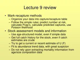
1. Lecture 9 review • Mark-recapture methods • Organize your data into capture/recapture table • Follow the simple rules: predict number at risk, calculate Pcap’s, calculate predicted captures, use Poisson likelihood • Stock assessment models and information • Use age-structured model, even if simple data • Get full catch history for the stock, even if catch estimates are crude • Try to get a current or recent estimate of U (F) • Fit to abundance trend data, with great suspicion • Do not rely upon extracting mortality information from age/size composition data

2. Why you should expect hyperstability in cpue data • Range contraction with effort targeted in areas of remaining high density • Concentration of effort in high cpue areas (scratch and mopup model) • Gear saturation effects (can’t handle more) at high abundances • Effort sorting (only the best keep fishing when abundance drops) • Covariation of effort with N in seasonal fisheries

3. N-E covariation in seasonal fisheries • Many fisheries are highly seasonal (eg shrimp), and deplete each season’s No down to some economic quitting abundance Ne. No changes from year to year, Ne tends to be stable • Annual catch in such cases is just C=No-Ne • Since N during season varies as N=Noe-qE, can predict E as E=-ln(Ne/No)/q • C/E then varies as (No-Ne)/(-ln(Ne/No)/q, which is NOT linear in No

4. N-E covariation in seasonal fisheries causes hyperstability • Plots of cpue=(total catch)/(total effort) show apparent density dependence in q:

5. Lecture 10: Designing effective sampling programs with many asides about crab assessment • When you measure something like fish density per area, there are two concerns: • Mean density • Total area to which this mean applies • Total area is called the “sampling universe” or “sampling frame” or “universe of inference” • Most sampling programs are designed without due care in defining the universe of inference (biologists focus on variability in density measurements)

6. The sampling universe • N is the sum over all units i of the abundance ni in each unit: N=Σni • N is also the mean ni times the number of sampling units in the universe Each little box is a sampling unit, has abundance ni

7. The sampling universe • To estimate N, remember that you must somehow assign an abundance ni to EVERY unit I, whether or not you could or did sample it • Your options include: • Assign mean of sampled ni to all unsampled units (assume your units are a random sample) • Sample units at regular spacing (grid) so as to uncover any spatial structure that may be present (take a systematic sample, whose mean will have lower variance than a random sample if and only if there is large-scale structure) • Assume structure in how the ni vary over space (or time), and try to estimate that structure (assign ni values to unsampled I) using spatial statistics models

8. What happens when you are not careful about defining the sampling universe: Australian NT mud crab example • Size frequency data give F estimates ranging from 0.5 to 5, depending on growth and vulnerability assumptions; either the fishery is barely touching the population, or is grossly overfishing it. • Depletion experiments (10, two areas, 1997-2004) to measure density, catchability (area swept by each trap)

9. Norm Hall’s model, gives F=4.5/year Carl’s GTG model, gives F=1.1/year (An aside about why you should not try to estimate fishing mortality rates from size-frequency data)

10. Another aside about why you should be fascinated by crab and shrimp fisheries • Apparent extreme resilience to fishing, but possibly due to a) bionomic shutdowns and b) invulnerable reserve stock • Very high economic value, growing importance even where finfish not depleted • Cannot age them and apply “standard” finfish assessment tools • Fast dynamics, so can see lots of changes

11. What happens when you are not careful about defining the sampling universe: Australian NT mud crab example • The depletion experiments have provided really neat results, showing size-selective depletion and recovery of aboundance over short time periods: • So we now know that one trap sweeps about 100 m2/day, i.e. a radius of about 5.6 m. • And we can then calculate the total area swept by traps per year • But q=(area per trap day)/(Total area)

12. What happens when you are not careful about defining the sampling universe: Australian NT mud crab example • We can then calculate the total area swept by traps per year (100m2 x Total trap days=128 million m2=100km2 • But q=(area per trap day)/(Total area), and F=q(Total trap days) or F=(total area swept)/(Total Area of stock) • What total area should we assume? Mud crabs are fished all along the 1200 km coastline of the “top end”, mainly in mangrove estuarine areas near major river mouths; the total area over which they are distributed could easily be less than 100km2

13. We also tried to to get around the q, F problem by fitting to monthly population model, but fits are excellent for wide range of q assumptions

14. What it would take to make the NT depletion data usable • Detailed coastal habitat maps (potential habitat area) • Detailed logbooks and/or surveys to determine distribution boundaries and concentration areas (e.g. FISHMAP), but as usual logbooks do not have accurate enough geo-referencing

15. Take a random sample, calculate variance σ2random among observations and sample mean Xran Take a systematic sample, calculate variance σ2systematic among observations and sample mean Xsyst Systematic vs random sampling (how would you map the NT mud crab distribution (“Universe”)?

16. Systematic vs random sampling (how would you map the NT mud crab distribution (“Universe”)? The fundamental theorem of systematic sampling says that systematic sample mean is more precise if σ2systematic>σ2random i.e. if the systematic sample deliberately inflates variance by crossing gradients

17. A common violation of the theorem is to take transects parallel to known gradients, rather than across them(without pre-defining strata) (What bonehead wildlife ecologists do in the Grand Canyon) (Whereas smart fish guys like Lauretta do it right, crossing gradient to maximize σ2)

18. The few vs many sites tradeoff • Typically multiple measurements are taken on each sampling unit:” important” y1,y2, … and “explanatory” x1, x2, x3 etc. • High cost and/or collaborator interest in the x’s typically leads to choosing few (or even just one) sites and measuring many things in these sites, on the assumption that the x’s are needed to explain (or capable of explaining) variation in the y’s. • But in complex systems, explanatory models based on the x’s generally fail (or cannot be validated) due to measuring y’s and x’s on too few sampling units. • The message: choose your y’s and x’s (and collaborators) carefully, and sample more sites. Do not expect to be able to predict successfully with data from one or a few sites, no matter how detailed the data are.

19. Examples of sampling too few sites intensively rather than many extensively (with careful variable choice) • Carnation creek salmon-logging study • Florida FIM program • Northern Territory mud crab depletions • LTER studies in general • IBP biome studies (except Polish and Russian Lake system studies)