Download
1 / 41
440 likes | 747 Vues
Neural Networks Chapter 8 Principal Components Analysis CS679 Lecture Note by Jahwan Kim Computer Science Department KAIST. Introduction. The purpose of an algorithm for self-organized learning or unsupervised learning is to discover features in the input data without a teacher.

E N D
Neural Networks Chapter 8 Principal Components Analysis CS679 Lecture Note by Jahwan Kim Computer Science Department KAIST
Introduction • The purpose of an algorithm for self-organized learning or unsupervised learning is to discover features in the input data without a teacher. • To do so, the algorithm is provided with rules of a local nature; the term “local” means that the change applied to the weight is confined to the immediate neighborhood of that neuron. • This chapter is restricted to Hebbian learning. The primary focus of the chapter is principal components analysis.
Some Intuitive Principles of Self-Organization • PRINCIPLE 1. Modifications in synaptic weights tend to self-amplify. • PRINCIPLE 2. Limitation of resources leads to competition among synapses and therefore the selection of the most vigorously growing synapses (i.e., the fittest) at the expense of the others. • PRINCIPLE 3. Modifications in synaptic weights tend to cooperate. • Note that all of the above three principles relate only to the neural network itself.
Intuitive Principles • PRINCIPLE 4. Order and structure in the activation patterns represent redundant information that is acquired by the neural network in the form of knowledge, which is a necessary prerequisite to self-organized learning. • Example: Linsker’s model of the mammalian visual system
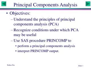
Principal Components Analysis • Goal: Find an invertible linear transformation T such that the truncation of Tx is optimum in the mean-squared error sense. • Principal components analysis provides the right answer.
PCA • The answer can be found by Lagrange multiplier method. We obtain the following: • Note that all eigenvalues are real and nonnegative since the correlation matrix is symmetric and positive semi-definite. More precisely, we have the following
PCA • (Finite-Dimensional, Baby) Spectral Theorem
PCA • Since the unit eigenvectors form an orthonormal basis of the data space, we can rewrite any vector in terms of this basis: • Then we approximate the data vector by truncating the expansion: • The approximation error vector is the difference of these two: • Note that the error vector is orthogonal to the approximating data vector. This is known as the principle of orthogonality.
PCA • The linear projecton given by truncation represents an encoder for the approximate representation of the data vector. See the figure.
Hebbian-Based Maximum Eigenfilter • A single liner neuron with a Hebbian-type adaptation rule can evolve into a filter for the first principal component of the input. • Formulation of the algorithm:
Maximum Eigenfilter • How do we derive the above algorithm from Hebb’s postulate of learning? • Hebb’s postulate can be written as • However, this rule leads to the unlimited growth of the weights. We may overcome this problem by incorporating saturation or normalization in the learning:
Maximum Eigenfilter • Expand this into power series in the learning parameter, and ignoring higher degree terms, • We may think of as the effective input. Then we may rewrite the above equation
Maximum Eigenfilter • We can rewrite the last equation by substituting the output value, and obtain a nonlinear stochastic difference equation: • Does our algorithm converge?
Maximum Eigenfilter • Consider a generic stochastic approximation algorithm: • We can (but won’t in detail) analyze the convergence of such algorithm by associating a deterministic ordinary differential equation to it.
Maximum Eigenfilter • Rough explanation: Assume certain conditions. See the textbook, page 407 for details. The key conditions are: • We maintain a savvy silence on what we mean by local asymptotical stability. See Chapter 14 if interested.
Maximum Eigenfilter • Asymptotic Stability Theorem. Under the above conditions, almost always. • We can check the maximum eigenfilter satisfies all of the conditions of the above theorem. • In summary, • The variance of the model output approaches the largest eigenvalue of the correlation matrix: • The synaptic weight vector of the model approaches the associated unit eigenvector:
Hebbian-Based Principal Components Analysis • Expanding a single linear neuron model into a feedforward network with a single layer of linear neurons, we can perform principal components analysis of arbitrary size. • Fix notations:
Hebbian-Based PCA • Generalized Hebbian Algorithm: • 1. Initialize the weights to a small random values at n=1. Assign a small positive value to the learning-rate parameter. • 2. Compute • 3. Increment n by 1, and go to step 2. Repeat until all synaptic weights reach their steady-state values.
Hebbian-Based PCA • The GHA computes weights convergent to the first l eigenvectors. The convergence can be proven as in the case of maximum eigenfilter. • Furthermore, in the limit, This equation may be viewed as one of data reconstruction.
Hebbian-Based PCA • Note that it is not necessary to compute the correlation matrix. The resulting computational savings can be enormous when m is very large, and l is a small fraction of m. • Although the convergence is proven for a time-varying learning-rate parameter, in practice we set the learning-rate parameter to a small constant.
Computer Experiment: Image Coding • See Figure 8.9 and 8.10 in the textbook. Scanned images won’t do any good for this.
Adaptive Principal Components Analysis Using Lateral Inhibition • Adaptive Principal Components Extraction (APEX) algorithm • Uses both feedforward and feedback (lateral) connections. • Feedforward connections are as in the case of GHA. • Lateral connections are inhibitory; the first (j-1) output neurons are connected to the j-th output neuron with weights • Iterative nature: Given the first (j-1) principal components, the j-th principal component is easily computed.
Adaptive PCA Using Inhibition • Summary of the APEX algorithm • 1. Initialize both feedforward and feedback weight vectors to a small random value at n=1, for all j. Assign a small positive value to the learning-rate parameter. • 2. Set j=1, and for n=1, 2, …, compute For large n, the weight vector will converge to the first eigenvector.
Adaptive PCA Using Inhibition • 3. Set j=2, and for n=1, 2, …, compute
Adaptive PCA Using Inhibition • 4. Increment j by 1, go to Step 3, and continue until j=m, where m is the desired number of principal components. • For large n, the j-th feedforward weight vector converges to the j-th eigenvalue, and the lateral weight vector to 0. • The optimal learning-rate parameter is However, a more practical proposition is • We skip the proof of convergence of the APEX algorithm.
Two Classes of PCA Algorithms • The various PCA algorithms can be categorized into two classes: reestimation algorithms and decorrelating algorithm. • Reestimation algorithm • Only feedforward connections • Weights are modified in Hebbian manner. • E.g., GHA • Decorrelating algorithm • Both feedforward and feedback connections • Forward connections follow a Hebbian law, whereas feedback connections follow an anti-Hebbian law. • E.g., APEX
Two Classes of PCA Algorithms • Principal subspace • Recall that GHA can be written as where the reestimator is • When only the principal subspace is required, we may use a symmetric model in which all the reestimator is replaced by
Two Classes of PCA Algorithms • In the symmetric model, the weight vectors converge to orthogonal vectors which span the principal subspace, rather than to the principal components themselves.
Batch and Adaptive Methods of Computation • Batch Methods: Direct eigendecomposition and the related method of singular value decomposition (SVD) • Direct eigendecomposition
Batch and Adaptive Methods • Better to use singular value decomposition theorem:
Batch and Adaptive Methods • Apply the SVD theorem to the data matrix Since we obtain • The singluar values of the data matrix are the sqaure rootsof the eigenvalues of the estimate of the correlation matrix. • The left singular vectors of the data matrix are the eigenvectors of the estimate.
Batch and Adaptive Methods • Adaptive Methods: GHA, the APEX algorithm • Work with arbitrarily large N. • Storage requirement is modest. • In a nonstationery environment, they have an inherent ability to track gradual changes in the optimal solution in an inexpensive way. • Drawback: slow rate of convergence
Kernel Principal Components Analysis • We perform PCA for these feature vectors. • As with ordinary PCA, we first assume the feature vectors have zero mean. Though not so simple, we can make this requirement satisfied. See Problem 8.10.
Summary • How useful is PCA? • For good data compression, PCA offers a useful self-organized learning procedure. • When a data set consists of several clusters, the principal axes found by PCA usually pick projections with good separation. PCA provides an effective basis for feature extraction in this case. See the figure. • Therefore, PCA is applicable as the preprocessor for a supervised network: Speed up convergence of the learning process by decorrelating the input data.
Summary • PCA doesn’t seem to be sufficient in biological perceptual systems.