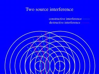
Two Point Source Interference Pattern
Two Point Source Interference Pattern. A Mathematical Analysis. 2 Point Interference Pattern. Nodal Lines. Nodes are areas of destructive interference and antinodes are the opposite (constructive) In standing waves, nodes are the particles that appear to stand still

Two Point Source Interference Pattern
E N D
Presentation Transcript
Two Point Source Interference Pattern A Mathematical Analysis
Nodal Lines • Nodes are areas of destructive interference and antinodes are the opposite (constructive) • In standing waves, nodes are the particles that appear to stand still • Nodal lines occur in areas of destructive interference (crest+trough or trough+crest) • Nodal lines in light interference would be dark • An antinodal line appears in the centre of an interference pattern when the two frequencies of the sources match) • The “count” of the nodal and antinodal lines increases as one moves away from the centre antinodal line
Point A, on antinodal line 1 PD = | S1A - S2A | = | 5 - 6 | = 1
Point B, on antinodal line 1 PD = | S1B - S2B | = | 3 - 4 | = 1
Point C, on antinodal line 2 PD = | S1C - S2C | = | 4 - 6 | = 2
Changing Notation Somewhat • Look only at nodal lines • Remember that nodal line numbers get larger as you move out from centre • The first nodal line is just to the right of the right bisector of the line joining the sources • Instead of A,B,C, etc., we will call the general point, P, and use a subscript to denote the nodal line on which it sits
Point D, on nodal line 1 PD = | P1S1 – P1S2 | = | 5–4.5 | = 0.5
Point E, on the nodal line 2 PD = | P2S1– P2S2| = | 3.5–5 | = 1.5
Blue: Nodal Lines Red: Antinodal Lines
General Relationship • Note that this is only for nodal lines (destructive interference) • Antinodal lines would have (n-1) instead PD = | PnS1 – PnS2 | =(n-0.5)l
Nodal Line Analysis • Where q is the angle for the nth nodal line from the main nodal line (right bisector) • l is the wavelength • d is the source spacing
Boundary Conditions • qn cannot be larger than 1, the RHS cannot be larger than 1 • The largest n that satifies this condition will be seen in the interference pattern – count them! • By measuring d and counting nodal lines, we can approximate l
Make note of what each variable means using the diagram to the right.
Example 1 • Two point sources generate identical waves that interfere in a ripple tank. The sources are located 5.0 cm apart, and the frequency of the waves is 8.0 Hz. A point on the first nodal line is located 10 cm from one source and 11 cm from the other. • What is the wavelength of the waves? • [2.0 cm/s] • What is the speed of the waves? • [16 cm/s]
Example 2 • A ripple tank experiment has given the following data from 2 point sources operating in phase: n=3, x3=35cm, L=77, d=6.0cm, q3=25°, 5 crests=4.2cm. Using 3 methods, determine the wavelength of the waves.