Download
1 / 40
400 likes | 556 Vues
Vertical Mixing Parameterizations and their effects on the skill of Baroclinic Tidal Modeling Robin Robertson Lamont-Doherty Earth Observatory of Columbia University Palisades, NY. Domain. Internal Wave Theory. Internal wave generation criteria according to linear theory

E N D
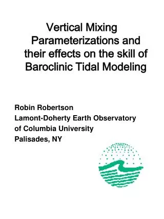
Vertical Mixing Parameterizations and their effects on the skill of Baroclinic Tidal Modeling Robin Robertson Lamont-Doherty Earth Observatory of Columbia University Palisades, NY
Internal Wave Theory • Internal wave generation criteria according to linear theory • - slope of internal wave rays • =1 – critical • Most generation • resonant • < 1 – subcritical • Less generation • Propagates both on and offslope • > 1 – supercritical • Less generation • Propagates offslope
Vertical Mixing Parameterizations • Large-McWilliams-Doney (LMD) Kp profile • Mellor-Yamada 2.5 level turbulence closure (MY2.5) • Brunt-Väisälä frequency (BVF) • Pacanowski-Philander (PP) • Generic Length Scale (GLS) • Lamont Ocean Atmosphere Mixed Layer Model (LOAM ) • LMD - modified
Large-McWilliams-Doney Kp profile • Primary processes • Local Ri instabilities due to resolvable vertical shear • If (1-Ri/0.7) > 0 10-3 (1-Ri/0.7)3 • Convection • N dependent 0.1 * [1.-(2x10⁻⁵ –N2)/2x10-5] • Internal wave • N dependent 10-6/N2 (min N of 10-7) • Double diffusion • Only for tracers • For Ri< 0.8, the first dominates • For Ri> 0.8, the third dominates • Modified • Non-local fluxes, Langmuir, Stokes drift • Changes two of the Kp profile values
Mellor-Yamada 2.5 level turbulence closure • Designed for boundary layer flows • Based on turbulent kinetic energy and length scale which are time stepped through the simulation • Matched laboratory turbulence • Logarithmic law of the wall • Not designed for internal wave mixing • Fails in the presence of stratification
Brunt-Väisälä frequency • Diffusivity is a function of N • If N < 0 Kv = 1 • If N = 0 Kv = background value • If N > 0 Kv = 10-7/N • Min of 3x10⁻⁵ • Max of 4x10⁻⁴ • Background values is input (10-6)
Pacanowski-Philander • Designed for the tropics • Gradient Ri dependent • If Ri > .2 Kv = 0.01/(1-5Ri)2+background max = 0.01 • Otherwise Kv = 0.01 • LOAM – version modified for use outside the tropics • If Ri > .2 Kv = 0.05/(1-5Ri)2+background max = 0.05 • Otherwise Kv = background
Generic Length Scale • Two generic equations • D - turbulent and viscous transport • P - KE production by shear • G - KE production by buoyancy • - Dissipation • c - model constants • Based on turbulent kinetic energy and length scale which are time stepped through the simulation • MY2.5 is a special case • p=0, m=1, n=1
Major Axis Errors Red indicated absolute error values lower than those of the base case.
Vertical Diffusivity Observations From Kunze et al. [1991]
Summary • Baroclinic tides were simulated using ROMS • Semidiurnal tides were reproduced successfully • Diurnal tides were not reproduced • Critical latitude effects • Mean currents insufficiently simulated • Generic Length Scale (GLS) produced the most realistic vertical diffusivities • Acknowledgments – Data from Brink, Toole, Kunze, Noble, and Eriksen
Model Description Regional Ocean Modeling System (ROMS) · Primitive equation model; non-linear Split 2-D and 3-D modes · Boussinesq and hydrostatic approximations · Horizontal advection - 3rd order upstream differencing [McWilliams and Shchepetkin] · Explicit vertical advection · Laplacian lateral diffusion along sigma surfaces (1 m2 s-1) · LMD scheme for vertical mixing Exact baroclinic pressure gradient · Density based on bulk modulus · Tidal Forcing – M2, S2, O1, and K1 Elevations - set at boundaries · 2-D velocities – radiation [Flather] · 3-D velocities – flow relaxation scheme · tracers – flow relaxation scheme · Time Step - 4 s barotropic, 120 s baroclinc mode · Simulation Duration: 30 days
Evaluation of Operational Considerations and Parameterizations • Horizontal Resolution: • Improving resolution improves agreement • 1 km shows best agreement • Vertical Resolution: • No. of Levels: • Doubling the number of levels from 30 to 60 slightly improved the agreement • Increasing the number of levels to 90, showed no improvement • Spacing: • Uneven spacing with more levels near the surface and bottom improves agreement with observations • Best match - shallow mixed layer, S = 2, and B = .5 • Bathymetry: • Improvement with the finer scale Eriksen bathymetry • Increased generation of internal tides on a small scale • Hydrography: • Improvement with the finer scale Kunze hydrography • Baroclinic Pressure Gradient: • Weighted Density Jacobian performed more poorly than Spline Density Jacobian • Vertical Mixing: • GLS showed the best agreement • Horizontal Mixing: No appreciable effect
Sensitivity Study • Bathymetry • Hydrography • Horizontal Resolution • Vertical Resolution and Spacing • Baroclinic Pressure Gradient Parameterization • Vertical Mixing Parameterization • Horizontal Mixing
Major Axis Errors Red indicated absolute error values lower than those of the base case.
Case Number Purpose Horizontal Resolution (x, y) Vertical Resolution no. of levels) Vertical Resolution: Spacing (mixed layer, S B) Baroclinic Pressure Gradient Vertical Mixing Horizontal Mixing Other 1 Base Case 2 km 60 uneven (100,2,.5) SDJ LMD 2nd Order Laplacian 2 Horizontal Resolution 4 km 30 uneven (100,2,.5) SDJ LMD 2nd Order Laplacian 3 Horizontal Resolution 1 km 60 uneven (100,2,.5) SDJ LMD 2nd Order Laplacian 4 Bathymetry 2 km 60 uneven (100,2,.5) SDJ LMD 2nd Order Laplacian Smith & Sandwell 5 Hydrography 2 km 60 uneven (100,2,.5) SDJ LMD 2nd Order Laplacian Kunze 6 Vertical Resolution 2 km 30 uneven (100,2,.5) SDJ LMD 2nd Order Laplacian 7 Vertical Resolution 2 km 90 uneven (100,2,.5) SDJ LMD 2nd Order Laplacian 8 Vertical Resolution 2 km 60 even (400, 1, 1) SDJ LMD 2nd Order Laplacian 9 Vertical Resolution 2 km 60 even (100, 1, 1) SDJ LMD 2nd Order Laplacian 10 Vertical Resolution 2 km 60 uneven (100, 2, 1) SDJ LMD 2nd Order Laplacian 11 Vertical Resolution 2 km 60 uneven (100, 4, 1) SDJ LMD 2nd Order Laplacian 12 Baroclinic Pressure Gradient 2 km 60 uneven (100,2,.5) Weighted Density Jacobian LMD 2nd Order Laplacian 13 Vertical Mixing 2 km 60 uneven (100,2,.5) SDJ Brünt-Väisäla Frequency 2nd Order Laplacian 14 Vertical Mixing 2 km 60 uneven (100,2,.5) SDJ Mellor-Yamada 2.5 Level Clos. 2nd Order Laplacian 15 Vertical Mixing 2 km 60 uneven (100,2,.5) SDJ Pacanowski-Philander 2nd Order Laplacian 16 Vertical Mixing 2 km 60 uneven (100,2,.5) SDJ LOAM 2nd Order Laplacian 17 Vertical Mixing 2 km 60 uneven (100,2,.5) SDJ LMD without BKPP 2nd Order Laplacian 18 Vertical Mixing 2 km 60 uneven (100,2,.5) SDJ LMD modified 2nd Order Laplacian 19 Vertical Mixing 2 km 60 uneven (100,2,.5) SDJ Generic Length Scale 2nd Order Laplacian 20 Horizontal Mixing 2 km 60 uneven (100,2,.5) SDJ LMD 1 m2 s-1 21 Horizontal Mixing 2 km 60 uneven (100,2,.5) SDJ LMD 1x10⁻⁶ m2 s-1 22 Other 2 km 60 uneven (100,2,.5) SDJ LMD 2nd Order Laplacian Latitude Shift 5oS Simulations