Download
1 / 40
400 likes | 530 Vues
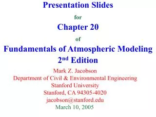
Presentation Slides for Chapter 13 of Fundamentals of Atmospheric Modeling 2 nd Edition. Mark Z. Jacobson Department of Civil & Environmental Engineering Stanford University Stanford, CA 94305-4020 jacobson@stanford.edu March 29, 2005. Sizes of Atmospheric Constituents.

E N D
Presentation SlidesforChapter 13ofFundamentals of Atmospheric Modeling 2nd Edition Mark Z. Jacobson Department of Civil & Environmental Engineering Stanford University Stanford, CA 94305-4020 jacobson@stanford.edu March 29, 2005
Sizes of Atmospheric Constituents Mode Diameter (mm) Number (#/cm3) Gas molecules 0.0005 2.45x10¹⁹ Aerosol particles Small < 0.2 103-106 Medium 0.2-2 1-104 Large 1-100 <1 - 10 Hydrometeor particles Fog drops 10-20 1-1000 Cloud drops 10-200 1-1000 Drizzle 200-1000 0.01-1 Raindrops 1000-8000 0.001-0.01 Table 13.1
Particles and Size Distributions Particle Agglomerations of molecules in the liquid and / or solid phases, suspended in air. Includes aerosol particles, fog drops, cloud drops, and raindrops Example 13.1. - Idealized particle size distribution 10,000 particles of radius between 0.05 and 0.5 m 100 particles of radius between 0.5 and 5.0 m 10 particles of radius between 5.0 and 50 m Example 13.2. Number of size bins needs to be limited 105 grid cells 100 size bins 100 components per size bin --> 109 words = 8 gigabytes to store concentration
Volume Ratio Size Structure Volume of particles in one size bin (13.1) (13.2) Volume-diameter relationship for spherical particles
Volume Ratio Size Structure Variation in particle sizes with the volume ratio size structure Fig. 13.1
Volume Ratio Size Structure Volume ratio of adjacent size bins (13.3) Example 13.3. d1 = 0.01 m = 1000 m NB = 30 size bins ---> Vrat = 3.29
Volume Ratio Size Structure Number of size bins (13.4) Example 13.4. d1 = 0.01 m = 1000 m Vrat = 4 --->NB = 26 size bins Vrat = 2 ---> NB = 51 size bins
Volume Ratio Size Structure Average volume in a size bin (13.5) Relationship between high- and low-edge volume (13.6) Substitute (13.6) into (13.5) --> low edge volume (13.7)
Volume Ratio Size Structure Volume width of a size bin (13.8) Diameter width of a size bin (13.9)
Particle Concentrations Number concentration in a size bin (13.10) Number concentration in a size distribution (13.11) Volume concentration in a size bin (13.12) Surface area concentration in a size bin (13.13)
Particle Concentrations Mass concentration in a size bin (13.14) Volume-averaged mass density (g cm-3) of particle of size i(13.15)
Particle Concentrations Example 13.5 = 3.0 g m-3 for water = 2.0 g m-3 for sulfate di= 0.5 m = 1.0 g cm-3 for water = 1.83 g cm-3 for sulfate ---> = 3 x 10-12 cm3 cm-3 for water ---> = 1.09 x 10⁻¹² cm3 cm-3 for sulfate ---> = 5.0 g m-3 ---> = 4.09 x 10⁻¹² cm3 cm-3 ---> = 6.54 x 10⁻¹⁴ cm3 ---> = 62.5 partic. cm-3 --->= 4.8 x 10⁻⁷ cm2 cm-3
Lognormal Distribution Bell-curve distribution on a log scale Geometric mean diameter 50% of area under a lognormal curve lies below it Geometric standard deviation 68% of area under a lognormal curve lies between +/-1 one geometric standard deviation around the mean diameter
Lognormal Distribution Describes particle concentration versus size dv (mm3 cm-3) / d log10 Dp Fig. 13.2a
Lognormal Distribution The lognormal curve drawn on a linear scale dv (mm3 cm-3) / d log10 Dp Fig. 13.2b
Lognormal Parameters From Data Low-pressure impactor -- 7 size cuts 0.05 - 0.075 m 0.5 - 1.0 m 0.075 - 0.12 m 1.0 - 2.0 m 0.12 - 0.26 m 2.0- 4.0 m 0.26 - 0.5 m
Lognormal Parameters From Data Natural log of geometric mean mass diameter (13.16) Total mass concentration of particles (g m-3)
Lognormal Parameters From Data Natural log of geometric mean volume diameter (13.17) Total volume concentration of particles (cm3 cm-3)
Lognormal Parameters From Data Natural log of geometric mean area diameter (13.18) Total area concentration of particles (cm2 cm-3)
Lognormal Parameters From Data Natural log of geometric mean number diameter (13.19) Total number concentration of particles (partic. cm-3)
Lognormal Parameters From Data Natural log of geometric standard deviation (13.20)
Redistribute With Lognormal Parameter Redistribute mass concentration in model size bin (13.21) Redistribute volume concentration (13.22) Redistribute area concentration (13.23)
Redistribute With Lognormal Parameter Redistribute number concentration (13.24) Exact volume concentration in a mode (13.25)
Lognormal Modes Number (partic. cm-3), area (cm2 cm-3), and volume (cm3 cm-3) concentrations distributed lognormally dx / d log10 Dp (x=n,a,v) Fig. 13.3
Lognormal Param. for Cont. Particles Nucleation Accumulation Coarse Parameter Mode Mode Mode sg 1.7 2.03 2.15 NL (particles cm-3) 7.7x10⁴ 1.3x10⁴ 4.2 DN (mm) 0.013 0.069 0.97 AL (mm2 cm-3) 74 535 41 DA (mm) 0.023 0.19 3.1 VL (mm3 cm-3) 0.33 22 29 DV (mm) 0.031 0.31 5.7 Table 13.2
Quadramodal Size Distribution Size distribution at Claremont, California, on the morning of August 27, 1987 Fig. 13.4
Marshall-Palmer Distribution Raindrop number concentration between di and di+Ddi(13.30) Ddin0= value of ni at di = 0 n0 = 8.0 x 10⁻⁶ partic. cm-3m-1 r = x Rm-1 R = rainfall rate (1-25 mm hr-1) Total number concentration and liquid water content
Marshall-Palmer Distribution Example 13.6. R = 5 mm hr-1 di = 1 mm di+Ddi = 2 mm ---> ni = 0.00043 partic. cm-3 ---> nT = 0.0027 partic. cm-3 ---> wL = 0.34 g m-3
Modified Gamma Distribution Number concentration (partic. cm-3) of drops in size bin i(13.30)
Modified Gamma Distribution Parameters Table 13.3
Modified Gamma Distribution Example 13.7. Find number concentration of droplets between 14 and 16 m in radius at base of a stratus cloud ---> ri = 15 m ---> Dri = 2 m ---> ni = 0.1506 partic. cm-3
Full-Stationary Size Structure Average single-particle volume in size bin (i) stays constant. When growth occurs, number concentration in bin (ni) changes. Advantages: • Covers wide range in diameter space with few bins • Nucleation, emissions, transport treated realistically Disadvantages: • When growth occurs, information about the original composition of the growing particle is lost. • Growth leads to numerical diffusion
Full-Stationary Size Structure Demonstration of a problem with the full-stationary size bin structure Fig. 13.5
Full-Moving Structure Number concentration (ni) of particles in a size bin does not change during growth; instead, single-particle volume (i) changes. Advantages: • Core volume preserved during growth • No numerical diffusion during growth Disadvantages: • Nucleation, emissions, transport treated unrealistically • Reordering of size bins required for coagulation
Full-Moving Structure Preservation of aerosol material upon growth and evaporation in a moving structure Fig. 13.6
Full-Moving Structure Particle size bin reordering for coagulation Fig. 13.7
Quasistationary Structure Single-particle volumes change during growth like with full-moving structure but are fit back onto a full-stationary grid each time step. Advantages and Disadvantages: • Similar to those of full stationary structure • Very numerically diffusive
Quasistationary Structure After growth, particles in bin i have volume i’, which lies between volumes of bins j and k Partition volume of i between bins j and k while conserving particle number concentration (13.32) and particle volume concentration (13.33) Solution to this set of two equations and two unknowns (13.34)
Moving-Center Structure Single-particle volume (i) varies between i,hi and i,lo during growth, but i,hi, i,lo, and di remain fixed. Advantages: • Covers wide range in diameter space with few bins • Little numerical diffusion during growth • Nucleation, emission, transport treated realistically Disadvantages: • When growth occurs, information about the original composition of the growing particle is lost
Moving-Center Structure Comparison of moving-center, full-moving, and quasistationary size structures during water growth onto aerosol particles to form cloud drops. dv (mm3 cm-3) / d log10 Dp Fig. 13.8