Download
1 / 39
390 likes | 694 Vues
"Supply creates its own demand". J.B. Say. Say's Law. Demand is never really the problem. Keynes. "Demand gets firms to increase Supply". Less spending leads to less output. wages and prices are not flexible.

E N D
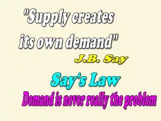
"Supply creates its own demand" J.B. Say Say's Law Demand is never really the problem
Keynes "Demand gets firms to increase Supply" Less spending leads to less output wages and prices are not flexible
“ I believe myself to be writing a book on economic theory which will largely revolutionize—not, I suppose, at once but in the course of the next ten years—the way the world thinks about economic problems. ” -- John Maynard Keynes The book, The General Theory of Employment, Interest, and Money, systematically analyzed the relationship between changes in aggregate expenditure and changes in GDP. In any particular year, the level of GDP is determined mainly by the level of aggregate expenditure.
Keynes' Equation: GDP = C + Ig + G + Xn or AE= C + Ig + G + Xn
C 0 GDP
Keynes' Equation: C GDP = C + Ig + G + Xn onsumption (by Households)
Consumption Real Consumption A smooth, upward trend, interrupted infrequently by brief recessions.
Consumption Current Disposable Income After taxes (-) and transfers (+) Household Wealth Every $1 increase increases consumption by 4-5 cents Expected Future Earnings Doesn’t seem to have much affect up or down Price Level Price levels affect real wealth more than total consumption Interest Rates Higher rates - more savings, lower rates - more consumption
Consumption and Savings S ____ ____ ____ ____ ____ ____ ____ ____ C 1540 1620 1700 1780 1860 1940 2020 2100 GDP 1500 1600 1700 1800 1900 2000 2100 2200
The Consumption Function Saving C Dis-saving Planned consumption(trillions of $) 45º line 12 9 6 3 45º Real disposable income(trillions of dollars) 3 6 9 12
Savings Consumption
The Relationship between Consumption and Income, 1960–2010 The line, which represents the relationship between consumption and disposable income, is called the consumption function. The slope of the consumption function is the marginal propensity to consume.
Marginal propensity to consume (MPC) The slope of the consumption function: The amount by which consumption spending changes when disposable income changes. Between 2006 and 2007, disposable income increased by $228 billion and consumption spending increased by $208 billion.
Marginal propensity to save (MPS) The amount by which saving changes when disposable income changes. Between 2006 and 2007, disposable income increased by $228 billion and if consumption spending increased by $208 billion, then savings increased by $20 billion. 1= MPC + MPS
Keynes' Equation: Ig GDP = C + Ig + G + Xn nvestment (gross) by Businesses
Planned Investment Real Investment
Investment Expectations of Future Profitability Interest Rates Higher rates - more savings, lower rates - more consumption Taxes Corporate taxes (-) Investment tax credits (+) Cash Flow The more profitable a firm is, the greater its cash flow and the greater its ability to finance investment.
The Consumption Function Saving C Dis-saving Unplanned Inventory Reduction Unplanned Increases in Inventory Planned consumption(trillions of $) 45º line 12 9 6 3 45º Real disposable income(trillions of dollars) 3 6 9 12
Keynes' Equation: G GDP = C + Ig + G + Xn overnment Expenditures a fixed amount
Keynes' Equation: GDP = C + Ig + G + Xn Xn Net eXports independent of income
Net Exports International Price Levels Lower inflation rates attract more consumption GDP Growth Rates Among Countries Higher incomes increase consumption The Exchange Rates Appreciating currency increases import consumption, but decreases export consumption.
Keynesianequilibrium AE = C AE = C + I + G AE = C + I + G + NX AE = C + I Full Employment(potential GDP) Planned aggregate expenditures(trillions of $) Equilibrium(AE= GDP) 10.3 10.0 9.7 45º Output(Real GDP -- trillions of $) 9.4 10.0 10.6 Keynes' Equilibrium
AE = C + I + G + NX, P3 AE = C + I + G + NX,P2 AE = C + I + G + NX,P1 Planned aggregate expenditures(trillions of $) (AE= GDP) Output at 3 Price Levels 10.6 10.0 9.4 Output(Real GDP -- trillions of $) 45º 9.4 10.0 10.6 P3 P2 P1 AD 9.4 10.0 10.6
The Multiplier • The Multiplier: A change in an spending (e.g. investment) leads to an even larger change in output and employment. • The multiplier is the number by which the initial change in spending is multiplied to obtain the total increase. • The size of the multiplier depends onhow much is spent of each increase. • The greater this %, the greater the effect
The Multiplier • injections will increase the size of the multiplier; • leakages will decrease the size of the multiplier,
3/4 3/4 3/4 3/4 3/4 3/4 3/4 Expenditure stage Additional income(dollars) Additional consumption(dollars) Marginal propensity to consume Round 1 1,000,000 750,000 562,500 Round 2 750,000 Round 3 562,500 421,875 421,875 316,406 Round 4 316,406 237,305 Round 5 949,219 711,914 All others Total 4,000,000 3,000,000 For simplicity (here) it is assumed that all additions to income are either spent domestically or saved. • The multiplier concept is based upon the proportion of additional income that households choose to spend (here assumed to be 75% = 3/4).
Multiplier Assume the people will spend .8 (80%) of a change in their income and the change in business investment is $10 (billion). Complete the table below. How much will they save? ______
1 M= 1 - %spent Higher Spending Means a Larger Multiplier Size of multiplier MPC 9/10 10.0 4/5 5.0 3/4 4.0 2/3 3.0 1/2 2.0 1/3 1.5 • As the spending % increases more and more money of every injection is spent (and so received as payment and then spent again, received as payment and spent again, etc.). • The effect is that for higher spending, higher multipliers result, specifically the relationship follows this equation:
Calculating the effect of the multiplier: change in the injection % not spent (saved) Change in investment % saved multiplier effect $10 20% ________ $10 10% ________ $10 25% ________ $20 20% ________
a. If the current output rate is $5,000, what will tend to happen to business inventories, future output, and employment? b. If the current output rate is $6,500, what will tend to happen to business inventories, future output and employment? c. What is the equilibrium rate of income of this economy? d. If the economy’s full employment rate of output is $6,000, will the rate of unemployment be high, low, or normal, assuming the current planned demand persisted into the future? e. What would happen if there was an increase in investment of $250?
Keynesian View of the Business Cycle • During a downturn, business pessimism, declining investment, and the multiplier principle combine to plunge the economy further toward recession. • During an economic upswing, business and consumer optimism and expanding investment interact with the multiplier to propel the economy to an inflationary boom. • The theory suggests that a market-directed economy, left to its own devices, will tend to fluctuate between economic recession and inflationary boom.
Keynesian View of the Business Cycle • Regulation of aggregate expenditures is the crux of sound macroeconomic policy according to the Keynesian view. • If we could assure aggregate expenditures large enough to achieve capacity output, but not so large as to result in inflation, the Keynesian view implies that maximum output, full employment, and price stability would be attained.