Difference Equations
This document explores the iterative solutions to causal difference equations, specifically focusing on the equation y[n] - (1/2)y[n-1] = x[n]. We derive the solutions iteratively using given initial conditions, with the example where x[n] = n^2u[n] and y[-1] = 16. We investigate BIBO stability by analyzing both the impulse response and the zero-state solution. Applicability of tools like Mathematica for solving these equations is discussed, and we provide a closed-form solution to give a holistic understanding of the system's behavior under specified conditions.

Difference Equations
E N D
Presentation Transcript
Iterative Solutions • Example: y[n] - ½ y[n-1] = x[n] How many initial conditions do we need? • For x[n] = n2u[n] and y[-1] = 16, causal system, y[n] = ½ y[n-1] + x[n] • Compute answer iteratively: y[0], y[1], … y[0] = ½ y[-1] + x[0] = ½ (16) + 0 = 8 y[1] = ½ (8) + (1)2 = 5 y[2] = 6.5 y[3] = 12.25 y[4] = 22.125
Stability • Is the system bounded-input bounded-output (BIBO) stable? y[n] - ½ y[n-1] = x[n] Impulse response is the output y[n] for input x[n] = d[n] Zero-state response ys[n] to input d[n] is1, 0.5, 0.25, …, for n = 0, 1, 2, … System appears to be BIBO stable. • x[n] = n2 u[n] is unbounded in amplitude as n goes to infinity
Example:y[n] - ½ y[n-1] = x[n] with y0[-1] = 16 Zero-input solution y0[n] - ½ y0[n-1] = 0 y0[n] = ½ y0[n-1] y0[n] = 8 (½)nu[n] 8, 4, 2, 1, ½, … Zero-state solution ys[n] - ½ ys[n-1] = n2 ys[0] = 0 ys[1] = (½) 0 + (1)2 = 1 ys[2] = (½) 1 + (2)2 = 4.5 Important identity Zero-Input, Zero-State Solutions
Complete Solution • Closed-form solution of impulse response Algebraic solution (not numerical or iterative solution) y[n] = zero-input solution + zero-state solution y[n] = y0[n] + ys[n] • Using Mathematica on example on previous slide Needs[ “DiscreteMath`Master`” ]; RSolve[ { y[n] - (1/2) y[n-1] == n^2,y[-1] == 16 }, y[n], n] • Complete solution (for non-negative n) y[n] = -14 ( n + 2 ) + 2 ( n + 2 ) ( n + 3 ) + 22 + 2 (½)n
Forms of Difference Equations • Anti-causal (advance operator form) • Causality requires MN Set M = N; delay input/output by N samples • Iterative solution 2N initial conditions (N initial conditions if causal input) Analysis Only Analysis and Implementation
Zero Input Response Slide by Prof. Adnan Kavak • Linear combination of characteristic modes